Frequentist Calibration Curves with curveRfreq

Ecosystem orientation

The curveR ecosystem consists of three packages that share a common data contract defined by curveRcore:

curveRcore — preprocessing pipelines, forward model functions, inverse back-calculation functions, analytical gradients, the calibration_result S3 class, and eligibility-gating logic shared across fitting engines.
curveRfreq (this package) — frequentist nonlinear least-squares (NLS) calibration via fit_calibration_freq() and its multi-curve wrapper fit_calibration_freq_multiplate().
curveRbayes — Bayesian calibration via Stan; produces the same calibration_result object so downstream code is engine-agnostic.

If you need a full frequentist-vs-Bayesian comparison, including LOO-CV model selection and posterior predictive checks, see the hub vignette vignette("curveR-ecosystem-overview"). This vignette covers curveRfreq alone, from raw assay data to calibrated concentrations with per-sample precision.

Data loading and preprocessing

The `bead_assay_example` dataset

curveRfreq ships a synthetic multi-plate bead-based immunoassay dataset that mirrors the structure expected by the fitting pipeline.

library(curveRfreq)   # also attaches curveRcore
library(ggplot2)

# Supplying package = "curveRfreq" makes data() work whether the package
# is fully installed, loaded via pkgload::load_all(), or being built by
# pkgdown — in all cases R knows exactly which data/ folder to search.
data(bead_assay_example, package = "curveRfreq")

# Top-level structure
str(bead_assay_example, max.level = 1)
#> List of 6
#>  $ standards      :'data.frame': 60 obs. of  8 variables:
#>  $ blanks         :'data.frame': 24 obs. of  7 variables:
#>  $ samples        :'data.frame': 120 obs. of  13 variables:
#>  $ curve_id_lookup:'data.frame': 6 obs. of  5 variables:
#>  $ response_var   : chr "mfi"
#>  $ indep_var      : chr "concentration"

The list contains six elements:

Element	Description
`standards`	60 rows × 8 cols. One row per standard well.
`blanks`	24 rows × 7 cols. Four blank wells per plate.
`samples`	120 rows × 13 cols. Patient samples at dilution 1:2000.
`curve_id_lookup`	6 rows × 5 cols. Maps integer `curve_id` to antigen / plate metadata.
`response_var`	`"mfi"` — name of the response column.
`indep_var`	`"concentration"` — name of the independent variable column.

The dataset spans two antigens (alpha and beta) × three replicate plates each, giving six curve_id values (1–6). The alpha curves were simulated with a Gompertz model; the beta curves with a 5PL model, reflecting realistic between-antigen variation in curve shape.

head(bead_assay_example$standards)
#>   curve_id stype sampleid well    dilution     mfi assay_response_variable
#> 1        1     S   STD_01   A1 1000.000000   109.4                     mfi
#> 2        1     S   STD_02   B1  333.333333   316.9                     mfi
#> 3        1     S   STD_03   C1  100.000000  1133.0                     mfi
#> 4        1     S   STD_04   D1   33.333333  4156.1                     mfi
#> 5        1     S   STD_05   E1   10.000000 12458.1                     mfi
#> 6        1     S   STD_06   F1    3.333333 18933.4                     mfi
#>   assay_independent_variable
#> 1              concentration
#> 2              concentration
#> 3              concentration
#> 4              concentration
#> 5              concentration
#> 6              concentration

bead_assay_example$curve_id_lookup
#>   curve_id antigen study_accession experiment_accession   plate
#> 1        1   alpha      SDYexample           EXPexample plate_1
#> 2        2   alpha      SDYexample           EXPexample plate_2
#> 3        3   alpha      SDYexample           EXPexample plate_3
#> 4        4    beta      SDYexample           EXPexample plate_1
#> 5        5    beta      SDYexample           EXPexample plate_2
#> 6        6    beta      SDYexample           EXPexample plate_3

Preprocessing with `curveRcore::preprocess_standards()`

curveRfreq does not preprocess data. All transforms — concentration computation, prozone correction, blank handling, and log10 transforms — must be applied upstream via curveRcore::preprocess_standards() (or its component functions). This clean separation means both curveRfreq and curveRbayes receive data on the identical fitting scale, making results directly comparable.

preprocess_standards() applies these steps in order:

compute_concentration() — converts the dilution column to absolute concentration using the known undiluted standard concentration, optionally log10-transforming the result.
correct_prozone() — dampens the hook (prozone) effect at high concentrations by compressing post-peak signal toward the peak.
perform_blank_operation() — applies one of five blank strategies: "ignored" (default), "included" (append as extra point), "subtracted", "subtracted_3x", or "subtracted_10x".
compute_log_response() — applies log10() to the response. Values ≤ 0 are floored to 1 % of the minimum positive value before transformation.

For the bead assay example, the undiluted standard concentration is 30 AU/mL (the highest point in the dilution series stored as dilution = 1/CONC):

std_raw   <- bead_assay_example$standards
blank_raw <- bead_assay_example$blanks

# Preprocess one curve at a time, then stack
std_preprocessed <- do.call(rbind, lapply(
  split(std_raw, std_raw$curve_id),
  function(df) {
    cid   <- df$curve_id[1]
    blanks_for_curve <- blank_raw[blank_raw$curve_id == cid, ]
    result <- curveRcore::preprocess_standards(
      data                = df,
      antigen_settings    = list(standard_curve_concentration = 30),
      response_variable   = "mfi",
      independent_variable = "concentration",
      is_log_response     = TRUE,
      blank_data          = blanks_for_curve,
      blank_option        = "subtracted",
      is_log_independent  = TRUE,
      apply_prozone       = TRUE
    )
    result$data
  }
))

# Both response and concentration are now on the log10 scale
head(std_preprocessed[, c("curve_id", "concentration", "mfi")])
#>     curve_id concentration      mfi
#> 1.1        1   -1.52287875 1.964654
#> 1.2        1   -1.04575749 2.476663
#> 1.3        1   -0.52287875 3.047580
#> 1.4        1   -0.04575749 3.616883
#> 1.5        1    0.47712125 4.094851
#> 1.6        1    0.95424251 4.276834

Key contract: After preprocess_standards(), the column named concentration holds log10-transformed concentration, and the response column (mfi here) holds log10-transformed MFI. These are the scales that fit_calibration_freq_multiplate() expects.

Fitting all curves with `fit_calibration_freq_multiplate()`

Function signature and argument reference

fit_calibration_freq_multiplate() is the recommended entry point. It splits the stacked preprocessed data by curve_id, calls fit_calibration_freq() for each, collects results into a calibration_result_multiplate object, and handles per-curve errors gracefully.


# , cache = TRUE
# Samples stay on the RAW response scale — log-transform is applied
# internally during back-calculation.
# Note: pcov_threshold, min_dynamic_range_log10, max_rel_se, and bound_tol
# are parameters of fit_calibration_freq() only; the multiplate wrapper
# uses the single-curve defaults (20, 0.5, 5.0, 1e-4) for every curve.
samples_raw <- bead_assay_example$samples

mp <- fit_calibration_freq_multiplate(
  standards          = std_preprocessed,
  blanks             = blank_raw,
  samples            = samples_raw,
  response_var       = "mfi",
  model_names        = c("logistic4", "gompertz4"),
  is_log_response    = TRUE,    # response was log10-transformed in preprocessing
  is_log_independent = TRUE,    # concentration is on the log10 scale
  std_curve_conc     = 30,      # undiluted standard concentration, raw scale
  fixed_a            = NULL,    # estimate lower asymptote freely
  cv_x_max           = 150,     # cap pcov at 150 %
  n_grid             = 200L,    # grid resolution
  grid_min_conc      = 1e-4,    # grid lower bound, raw scale
  grid_max_conc      = NULL,    # NULL → uses std_curve_conc
  on_error           = "stop",   # DIAGNOSTIC: show actual error
  verbose            = TRUE      # DIAGNOSTIC: show fitting details
)
#> [1/6] curve_id=1
#> [constraints] scale=high, dr=2.356, slope=[0.100,2.000], g=[0.50,5.00]
#> 
#>  Trying model: logistic4
#>   ✓ logistic4 converged (AIC=-27.76)
#> 
#>  Trying model: gompertz4
#>   ✓ gompertz4 converged (AIC=-10.72)
#>   [eligibility] logistic4      ✓ eligible
#>   [eligibility] gompertz4      ✗ ineligible
#>     gate at_bound         a at upper bound
#>     gate dynamic_range    dynamic range = 0 log10 (need >= 0.5)
#>   [selection] best = logistic4
#> Waiting for profiling to be done...
#> [detection_limits] curve_id=1  LLOD_resp=1.904  ULOD_resp=4.299  MDC=[-1.686, 1.408]  RDL=[-1.676, 1.058]
#> [2/6] curve_id=2
#> [constraints] scale=high, dr=2.547, slope=[0.100,2.000], g=[0.50,5.00]
#> 
#>  Trying model: logistic4
#>   ✓ logistic4 converged (AIC=-19.17)
#> 
#>  Trying model: gompertz4
#>   ✓ gompertz4 converged (AIC=-16.12)
#>   [eligibility] logistic4      ✓ eligible
#>   [eligibility] gompertz4      ✗ ineligible
#>     gate dynamic_range    dynamic range = 0 log10 (need >= 0.5)
#>   [selection] best = logistic4
#> Waiting for profiling to be done...
#>   [warning] NaNs produced
#> [detection_limits] curve_id=2  LLOD_resp=1.791  ULOD_resp=4.237  MDC=[-1.513, 1.337]  RDL=[-1.493, 0.9289]
#> [3/6] curve_id=3
#> [constraints] scale=high, dr=2.381, slope=[0.100,2.000], g=[0.50,5.00]
#> 
#>  Trying model: logistic4
#>   ✓ logistic4 converged (AIC=-24.74)
#> 
#>  Trying model: gompertz4
#>   ✓ gompertz4 converged (AIC=-19.38)
#>   [eligibility] logistic4      ✓ eligible
#>   [eligibility] gompertz4      ✗ ineligible
#>     gate dynamic_range    dynamic range = 0 log10 (need >= 0.5)
#>   [selection] best = logistic4
#> Waiting for profiling to be done...
#> [detection_limits] curve_id=3  LLOD_resp=1.912  ULOD_resp=4.3  MDC=[-1.624, 1.285]  RDL=[-1.611, 0.9333]
#> [4/6] curve_id=4
#> [constraints] scale=high, dr=4.483, slope=[0.100,2.000], g=[0.50,5.00]
#> 
#>  Trying model: logistic4
#>   ✓ logistic4 converged (AIC=-4.17)
#> 
#>  Trying model: gompertz4
#>   ✓ gompertz4 converged (AIC=-1.58)
#>   [eligibility] logistic4      ✗ ineligible
#>     gate dynamic_range    dynamic range = 0 log10 (need >= 0.5)
#>   [eligibility] gompertz4      ✗ ineligible
#>     gate rel_se           c: rel_se=44.29
#>     gate dynamic_range    dynamic range = 0 log10 (need >= 0.5)
#>   [selection] best = logistic4 [fallback]
#> Waiting for profiling to be done...
#> [detection_limits] curve_id=4  LLOD_resp=0.133  ULOD_resp=4.338  MDC=[-1.158, 2.04]  RDL=[-1.12, 1.608]
#> [5/6] curve_id=5
#> [constraints] scale=high, dr=4.422, slope=[0.100,2.000], g=[0.50,5.00]
#> 
#>  Trying model: logistic4
#>   ✓ logistic4 converged (AIC=4.28)
#> 
#>  Trying model: gompertz4
#>   ✓ gompertz4 converged (AIC=-0.62)
#>   [eligibility] logistic4      ✗ ineligible
#>     gate dynamic_range    dynamic range = 0 log10 (need >= 0.5)
#>   [eligibility] gompertz4      ✗ ineligible
#>     gate dynamic_range    dynamic range = 0 log10 (need >= 0.5)
#>   [selection] best = gompertz4 [fallback]
#> Waiting for profiling to be done...
#> [detection_limits] curve_id=5  LLOD_resp=0.190  ULOD_resp=4.229  MDC=[-0.5996, 1.928]  RDL=[-0.5841, 1.485]
#> [6/6] curve_id=6
#> [constraints] scale=high, dr=4.444, slope=[0.100,2.000], g=[0.50,5.00]
#> 
#>  Trying model: logistic4
#>   ✓ logistic4 converged (AIC=18.69)
#> 
#>  Trying model: gompertz4
#>   ✓ gompertz4 converged (AIC=16.92)
#>   [eligibility] logistic4      ✗ ineligible
#>     gate at_bound         a at upper bound
#>     gate dynamic_range    dynamic range = 0 log10 (need >= 0.5)
#>   [eligibility] gompertz4      ✗ ineligible
#>     gate at_bound         a at upper bound; b at upper bound
#>     gate dynamic_range    dynamic range = 0 log10 (need >= 0.5)
#>   [selection] best = gompertz4 [fallback]
#> Waiting for profiling to be done...
#>   [warning] NaNs produced
#>   [warning] NaNs produced
#>   [warning] NaNs produced
#>   [warning] NaNs produced
#>   [warning] NaNs produced
#>   [warning] NaNs produced
#> [detection_limits] curve_id=6  LLOD_resp=0.992  ULOD_resp=3.815  MDC=[-0.1745, 1.098]  RDL=[-0.1337, 0.7864]

Argument reference

Argument	Type	Default	Meaning
`standards`	data frame	—	Required. Stacked preprocessed standards with `curve_id`, `concentration`, and the response column.
`blanks`	data frame	—	Required. Stacked blank data with `curve_id` and the response column, on the same fitting scale as `standards`. Stored in `result$blanks` for QA and plotting. Every `curve_id` in `standards` should have a corresponding entry.
`samples`	data frame or NULL	`NULL`	Stacked sample data on the raw (untransformed) response scale. The `dilution` column is used to recover pre-dilution concentration.
`response_var`	character	—	Required. Name of the response column. Must match what preprocessing produced.
`model_names`	character vector	`c("logistic4", "gompertz4")`	Which nonlinear models to fit. Any subset of `curveRcore::available_models()` is valid. `"loglogistic4"` is silently dropped when `is_log_independent = TRUE` because it is algebraically redundant with `"logistic4"` on the log scale.
`is_log_response`	logical	`TRUE`	Was the response log10-transformed during preprocessing? Must match the preprocessing step.
`is_log_independent`	logical	`TRUE`	Was concentration log10-transformed? Must match the preprocessing step.
`std_curve_conc`	numeric	—	Required. The undiluted standard concentration on the raw scale (e.g. 30 AU/mL). Used to generate the prediction grid.
`fixed_a`	numeric or NULL	`NULL`	If non-NULL, pins the lower asymptote `a` to this value (on the fitting scale, i.e. already log10-transformed if `is_log_response = TRUE`). When NULL, `a` is freely estimated. Fixing `a` is most useful when blank wells reliably define the lower asymptote.
`cv_x_max`	numeric	150	Hard cap on the percent coefficient of variation (%CV) of back-calculated concentration. Values above this threshold are set to `cv_x_max` in `$pcov` and `$pcov_rmse`.
`n_grid`	integer	200	Number of evenly spaced log10-concentration points on the prediction grid.
`grid_min_conc`	numeric	1e-4	Lower end of the prediction grid, raw scale.
`grid_max_conc`	numeric or NULL	`NULL`	Upper end of the prediction grid, raw scale. NULL uses `std_curve_conc`.
`curve_ids`	vector or NULL	`NULL`	Subset of `curve_id` values to fit. NULL fits all curves found in `standards`.
`on_error`	`"warn"` or `"stop"`	`"warn"`	Error handling per curve. `"warn"` stores NULL for the failed curve and continues; `"stop"` raises immediately.
`verbose`	logical	`FALSE`	Emit per-model convergence messages and eligibility gate results.

Note: pcov_threshold (default 20), min_dynamic_range_log10 (default 0.5), max_rel_se (default 5.0), and bound_tol (default 1e-4) are parameters of fit_calibration_freq() and are not exposed by the multiplate wrapper — the single-curve defaults are used for every curve. To override them, call fit_calibration_freq() directly for individual curves. —

The multi-start NLS algorithm and constraint system

Understanding the fitting engine helps interpret convergence failures and tune the algorithm for unusual assay configurations.

Adaptive parameter bounds

Before any fitting, compute_model_constraints() calls curveRcore::adaptive_constraint_profile(), which inspects the preprocessed response range and classifies the assay into one of three scale classes:

Scale class	Criterion (log response)	Typical assay
`"high"`	log10(MFI) max > 2.5	Luminex / bead-based
`"medium"`	log10(MFI) max > 0.5	Mid-range ELISA
`"low"`	log10(MFI) max ≤ 0.5	Absorbance / OD

The scale class drives the width of parameter bounds, which differ systematically:

Parameter	Role	`"high"` bounds	`"low"` bounds
`a`	Lower asymptote	`[y_min − 0.5·dr, y_min + 0.1·dr]`	same formula, narrower dr
`b`	Slope / steepness	`[0.1, 2.0]`	`[0.01, 5.0]` — wider to avoid singular Jacobians
`c`	Inflection point	±0.5 × conc range	±1.0 × conc range
`d`	Upper asymptote	`[y_min + 0.5·dr − margin, y_max + margin]` where margin = 0.5·dr	margin = 0.15·dr
`g`	Asymmetry (5PL)	`[0.5, 5.0]`	`[0.1, 10.0]`

The bound on a is only computed when fixed_a = NULL; otherwise a is not a free parameter and no bounds are needed.

Multi-start Levenberg-Marquardt

fit_ensemble_nls() fits each model independently. For each model it:

Generates starting values from generate_start_lists(). Candidate starts are evenly spaced across the parameter bounds:
- 3 starts for "high" and "medium" scale data.
- 5 starts for "low" scale data, with the slope b biased toward the lower end of its range (squared fractional spacing) to avoid overshooting the flat portion of low-signal curves.
Runs minpack.lm::nlsLM() for each start, keeping the fit with the lowest AIC. Tighter tolerances (ftol = ptol = 1e-8, maxiter = 200) are used for low-signal data.
Falls back if all primary starts fail and the scale class is "low":
- Fallback 1 — relaxes bounds by 50 % in each direction and retries nlsLM from the midpoint.
- Fallback 2 — switches to stats::nls() with algorithm = "port" (box-constrained trust-region), which can converge where Levenberg-Marquardt does not.

A model that exhausts all fallbacks is recorded with converged = FALSE and is excluded from downstream eligibility assessment and selection.

# Check convergence status for curve_id 1
cr1 <- mp$plates[["1"]]

convergence <- sapply(cr1$ensemble, function(e) {
  c(model = e$model_name, converged = e$converged)
})
t(convergence)
#>           model       converged
#> logistic4 "logistic4" "TRUE"   
#> gompertz4 "gompertz4" "TRUE"

The eligibility-gated AIC model selection pipeline

Why eligibility gates matter

AIC and other information criteria measure forward-fit quality: how well the model predicts the response values in the training data. They are completely blind to whether the fitted model can back-calculate concentration reliably. A model whose asymptote estimate has hit a constraint boundary, or whose covariance matrix is nearly singular, can have a lower AIC than a better-identified competitor purely by overfitting.

The eligibility gates intercept such models before they can be selected. Only models that pass all applicable gates enter the AIC ranking.

The four gates

All four gates are evaluated per model using curveRcore::assess_model_eligibility():

Gate 1 — `at_bound`

(Frequentist only; skipped when constraints = NULL)

Checks that no parameter estimate lies within bound_tol (default 1e-4) of its lower or upper constraint bound. A boundary solution means the optimiser could not find an interior minimum; AIC asymptotics do not hold at the boundary, and the resulting parameter estimates are not maximum-likelihood estimates in the usual sense.

Gate 2 — `vcov_condition`

(Frequentist only; skipped when vcov(fit) fails)

Computes the condition number κ of vcov(fit). If κ ≥ 1×10⁸, the covariance matrix is near-singular, making standard error propagation unreliable. This gate catches cases where two parameters are near-collinear — for example, when the inflection point c lies far outside the data range.

Gate 3 — `rel_se`

(Both frequentist and Bayesian)

Checks that SE / |estimate| < max_rel_se (default 5.0) for every free parameter. A relative SE larger than the estimate itself indicates an unidentified parameter — the data do not constrain it. This gate uses std_error from the NLS summary (frequentist) or sd from the posterior (Bayesian).

Gate 4 — `dynamic_range`

(Requires pcov_profile and grid_x)

Evaluates the precision grid (see Section 7) to locate the LLOQ and ULOQ — defined as the grid points where pcov crosses pcov_threshold (default 20 %) at the lower and upper ends, respectively. The gate passes if ULOQ − LLOQ ≥ min_dynamic_range_log10 (default 0.5 log10 units, approximately 3-fold). A model with zero quantifiable range is operationally useless even if it converged.

Selection logic

After assessment, curveRcore::select_best_eligible() implements the following decision tree:

eligible_models ← {models that passed all gates}

if length(eligible_models) > 0:
    best ← eligible_models ranked by AIC (lowest wins)
    fallback ← FALSE

else:                                        # fallback path
    best ← model with widest dynamic_range_log10;
            ties broken by AIC
    fallback ← TRUE
    fallback_reason ← per-model gate failure summary

The fallback ensures that a result is always returned. When fallback = TRUE the selection is a best-effort choice and should be treated with caution.

Reading the selection audit trail

The $selection component of each calibration_result contains the complete audit trail.

sel <- cr1$selection

# Was a fallback used?
sel$fallback
#> [1] FALSE
sel$fallback_reason   # empty string when fallback = FALSE
#> [1] ""

# Which models passed all gates?
sel$eligible_models
#> [1] "logistic4"

# The winning model
sel$best_model_name
#> [1] "logistic4"

# AIC comparison table (always computed, even for ineligible models)
sel$weights
#>   model_name converged       aic delta_aic       weight
#> 1  gompertz4      TRUE -10.72491  17.03944 0.0001994559
#> 2  logistic4      TRUE -27.76435   0.00000 0.9998005441

Per-model gate results

Every model in the ensemble carries its own eligibility report inside ensemble[[model]]$eligibility:

for (nm in names(cr1$ensemble)) {
  elig <- cr1$ensemble[[nm]]$eligibility
  cat(sprintf("\n── %s  (eligible = %s) ──\n", nm, elig$eligible))
  print(elig$gates)
  cat(sprintf(
    "   LLOQ = %.3f  ULOQ = %.3f  DR = %.3f log10\n",
    elig$lloq, elig$uloq, elig$dynamic_range_log10
  ))
}
#> 
#> ── logistic4  (eligible = TRUE) ──
#>             gate passed                     detail
#> 1       at_bound   TRUE                           
#> 2 vcov_condition   TRUE                           
#> 3         rel_se   TRUE                           
#> 4  dynamic_range   TRUE dynamic range = 1.76 log10
#>    LLOQ = -1.443  ULOQ = 0.322  DR = 1.765 log10
#> 
#> ── gompertz4  (eligible = FALSE) ──
#>             gate passed                                detail
#> 1       at_bound  FALSE                      a at upper bound
#> 2 vcov_condition   TRUE                                      
#> 3         rel_se   TRUE                                      
#> 4  dynamic_range  FALSE dynamic range = 0 log10 (need >= 0.5)
#>    LLOQ = NA  ULOQ = NA  DR = 0.000 log10

The `aic_best` field

The selection object also exposes $aic_best, the model name that would have been chosen by pure AIC (ignoring eligibility gates). When aic_best != best_model_name, the AIC winner was demoted by a gate failure — a useful diagnostic:

cat("AIC winner:         ", sel$aic_best, "\n")
#> AIC winner:          logistic4
cat("Eligibility winner: ", sel$best_model_name, "\n")
#> Eligibility winner:  logistic4

Per-model precision grids from `ensemble[[model]]$grid`

Grid computation — every converged model, not just the best

A critical design point: precision grids are computed for every converged model, not only the one ultimately selected. This happens in step 6a of fit_calibration_freq(), before eligibility assessment:

# Conceptually (internal to fit_calibration_freq):
ensemble_grids <- lapply(names(ensemble_raw), function(nm) {
  if (!ensemble_raw[[nm]]$converged) return(NULL)
  predict_grid_freq(grid = base_grid, fit = ensemble_raw[[nm]]$fit, ...)
})

The per-model grids are what feed the dynamic_range gate. After fitting, each grid is attached to its ensemble entry as ensemble[[model]]$grid. The top-level $grid slot of the calibration_result is simply a pointer to the best-model grid — no recomputation occurs.

Grid columns

grid_best <- cr1$grid
names(grid_best)
#>  [1] "log10_concentration"     "concentration"          
#>  [3] "x_fit"                   "predicted_response"     
#>  [5] "ci_lower"                "ci_upper"               
#>  [7] "predicted_concentration" "se_concentration"       
#>  [9] "pcov"                    "pcov_rmse"              
#> [11] "pcov_pass"               "d2y_dx2"

Column	Description
`x_fit`	Grid point on the fitting scale (log10 concentration, if `is_log_independent = TRUE`).
`log10_concentration`	Same as `x_fit` when `is_log_independent = TRUE`.
`predicted_response`	Forward model prediction: `ŷ = f(x, θ̂)`. On the fitting (log10) scale.
`ci_lower`, `ci_upper`	Delta-method 95 % CI on the response scale.
`predicted_concentration`	Back-calculated concentration from `ŷ`. On the fitting scale.
`se_concentration`	Delta-method SE of the back-calculated concentration.
`pcov`	Percent CV of back-calculated concentration (%). Capped at `cv_x_max`.
`pcov_rmse`	Relative RMSE (%) — includes bias of `predicted_concentration` vs `x_fit`.
`pcov_pass`	Logical. `TRUE` when `pcov < cv_x_max` and `pcov` is finite.

The `pcov` formula

For a log10-scale independent variable, pcov is computed from the delta-method SE on the log10 scale:

$\text{pcov} = \text{SE}_{x} \times \ln(10) \times 100 \%$

where $\text{SE}_x^2 = \nabla_\theta x^\top \Sigma \nabla_\theta x + \left(\frac{\partial x}{\partial y}\right)^2 \sigma_y^2$ and $\sigma_y$ is summary(fit)$sigma (residual SE of the response on the fitting scale). The first term captures parameter uncertainty (propagated through the inverse function via curveRcore::make_inv_and_grad_fixed()), and the second captures observation-level noise.

Comparing grids across models

Because every converged model has a grid, you can compare precision profiles side by side — even for the non-selected model:

library(ggplot2)

grid_list <- lapply(names(cr1$ensemble), function(nm) {
  g <- cr1$ensemble[[nm]]$grid
  if (is.null(g) || !"x_fit" %in% names(g)) return(NULL)
  g <- as.data.frame(g)  # explicit copy — prevents mutation of cr1$grid
  g$model <- nm
  g
})
grid_compare <- do.call(rbind, Filter(Negate(is.null), grid_list))

if (!is.null(grid_compare) && "x_fit" %in% names(grid_compare)) {
  ggplot(grid_compare,
         aes(x = x_fit, y = pcov, colour = model)) +
    geom_line(linewidth = 0.9) +
    geom_hline(yintercept = 20, linetype = "dashed", colour = "grey40") +
    annotate("text", x = -3.8, y = 22, label = "pcov threshold (20 %)",
             hjust = 0, size = 3.2, colour = "grey40") +
    scale_colour_manual(values = c(logistic4 = "#0072B2", gompertz4 = "#D55E00")) +
    labs(x = "log10 concentration", y = "Percent CV (%)",
         title = "Precision profiles — curve_id 1",
         colour = "Model") +
    theme_bw(base_size = 12)
} else {
  message("Skipping compare-grids plot: x_fit not available in ensemble grids.")
}
#> Warning: Removed 53 rows containing missing values or values outside the scale range
#> (`geom_line()`).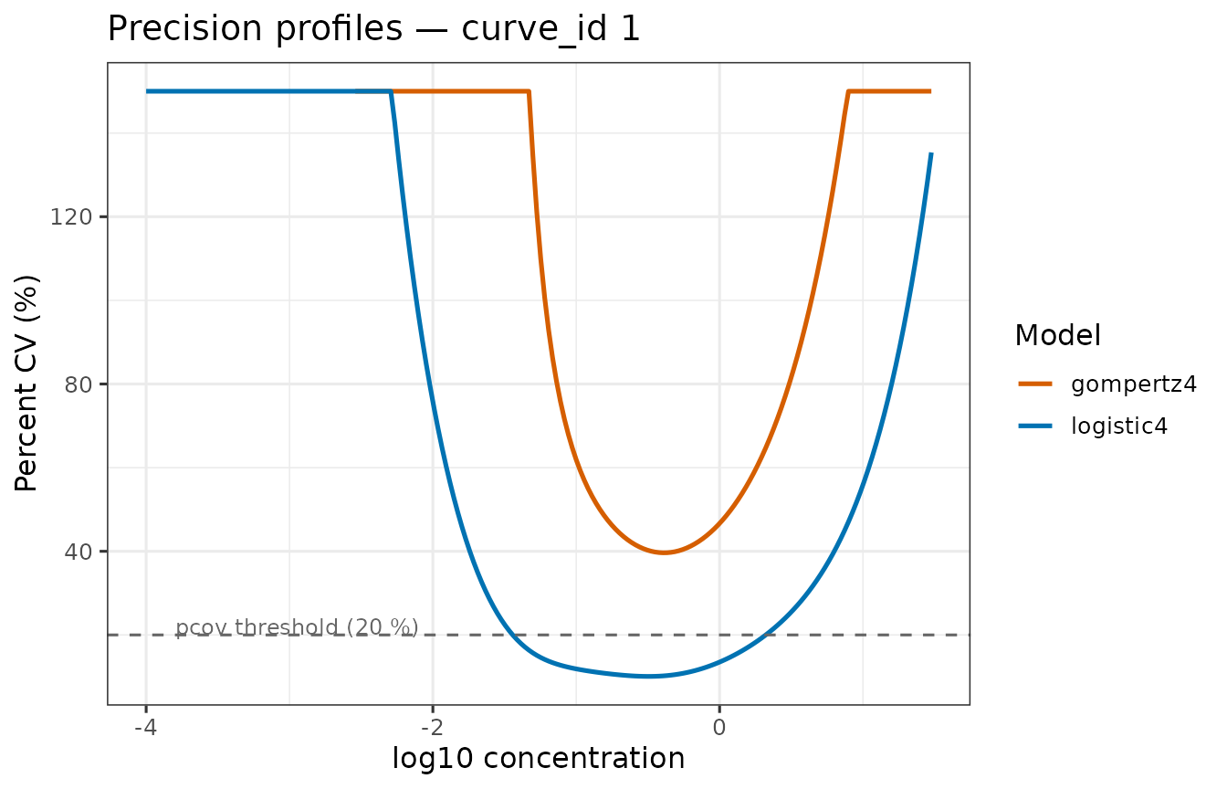

Precision profiles for both candidate models on curve_id 1.

Dynamic range, LLOQ, and ULOQ

Reading LOQ values from the eligibility report

The LLOQ and ULOQ (on the log10 concentration scale) are stored inside ensemble[[model]]$eligibility:

elig_best <- cr1$ensemble[[sel$best_model_name]]$eligibility

lloq_log10 <- elig_best$lloq
uloq_log10 <- elig_best$uloq
dr_log10   <- elig_best$dynamic_range_log10

cat(sprintf("LLOQ = %.3f log10 (%.4f AU/mL)\n", lloq_log10, 10^lloq_log10))
#> LLOQ = -1.443 log10 (0.0361 AU/mL)
cat(sprintf("ULOQ = %.3f log10 (%.3f  AU/mL)\n", uloq_log10, 10^uloq_log10))
#> ULOQ = 0.322 log10 (2.098  AU/mL)
cat(sprintf("Dynamic range = %.3f log10 units (%.1f-fold)\n",
            dr_log10, 10^dr_log10))
#> Dynamic range = 1.765 log10 units (58.2-fold)

Visualising the quantifiable range

# Build a fresh plain data frame to avoid any reference or class issues
g_best <- data.frame(
  x_fit = cr1$grid[["x_fit"]],
  pcov  = cr1$grid[["pcov"]]
)

ggplot(g_best, aes(x = x_fit, y = pcov)) +
  annotate("rect",
           xmin = lloq_log10, xmax = uloq_log10,
           ymin = -Inf,       ymax = Inf,
           fill = "#009E73", alpha = 0.12) +
  geom_line(colour = "#0072B2", linewidth = 1) +
  geom_hline(yintercept = 20, linetype = "dashed", colour = "grey40") +
  geom_vline(xintercept = c(lloq_log10, uloq_log10),
             linetype = "dotted", colour = "#009E73", linewidth = 0.8) +
  annotate("text", x = lloq_log10, y = 145, label = "LLOQ",
           hjust = -0.1, size = 3.5, colour = "#009E73") +
  annotate("text", x = uloq_log10, y = 145, label = "ULOQ",
           hjust = 1.1,  size = 3.5, colour = "#009E73") +
  coord_cartesian(ylim = c(0, 155)) +
  labs(x = "log10 concentration (AU/mL)",
       y = "Percent CV (%)",
       title = paste("Precision profile —", sel$best_model_name,
                     "— curve_id 1")) +
  theme_bw(base_size = 12)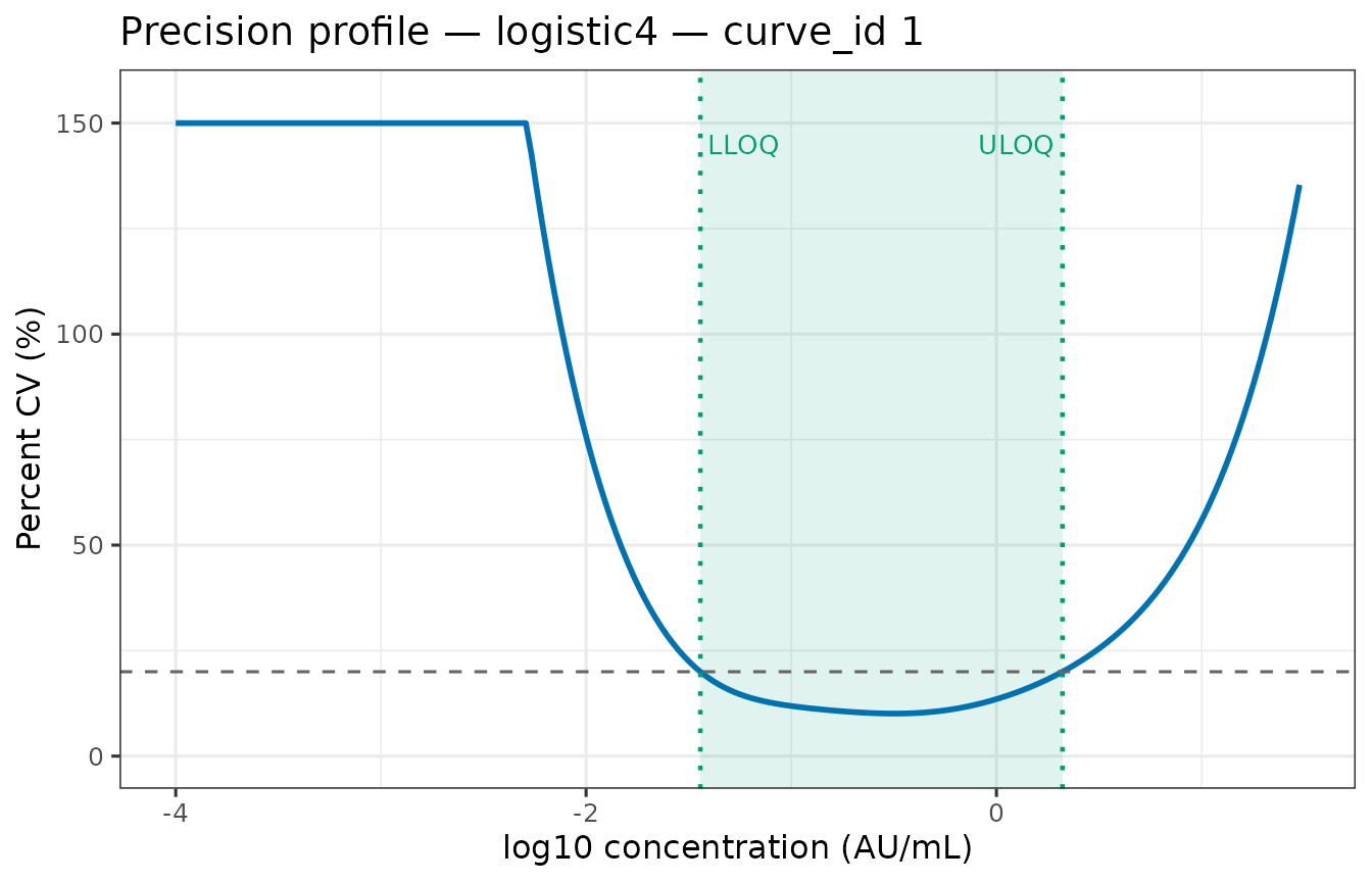

Precision profile with LLOQ and ULOQ indicated. The shaded region is the quantifiable range.

Interpretation: Any sample whose back-calculated concentration falls between LLOQ and ULOQ (shaded region) has a back-calculation %CV ≤ 20 %. Samples outside this range should be flagged or re-measured at a different dilution.

Detection limits, shape-LOQ, and the second derivative profile

Second derivative and curvature-based LOQ

In addition to the precision-profile-based LLOQ/ULOQ (derived from pcov threshold crossings), every per-model grid now includes a d2y_dx2 column: the second derivative $d^2(\log_{10} y) / d(\log_{10} x)^2$ , computed from the existing grid points with zero additional model evaluations.

The second derivative of a monotone increasing sigmoid has a peak below the inflection point, a zero crossing at the inflection point, and a valley above it. The shape-LLOQ (peak) and shape-ULOQ (valley) bracket the quasi-linear region of maximum assay sensitivity.

These are stored in ensemble[[model]]$eligibility as shape_lloq_log10, shape_uloq_log10, and their natural-scale and response-scale counterparts.

best_grid <- as.data.frame(cr1$ensemble[[sel$best_model_name]]$grid)
best_elig <- cr1$ensemble[[sel$best_model_name]]$eligibility

if ("d2y_dx2" %in% names(best_grid)) {
  ok <- is.finite(best_grid$d2y_dx2)

  ggplot(best_grid[ok, ],
         aes(x = x_fit, y = d2y_dx2)) +
    geom_line(colour = "#0072B2", linewidth = 1) +
    geom_hline(yintercept = 0, linetype = "dashed", colour = "grey40") +
    {if (is.finite(best_elig$shape_lloq_log10))
      geom_vline(xintercept = best_elig$shape_lloq_log10,
                 linetype = "dotted", colour = "#D55E00", linewidth = 0.8)} +
    {if (is.finite(best_elig$shape_uloq_log10))
      geom_vline(xintercept = best_elig$shape_uloq_log10,
                 linetype = "dotted", colour = "#D55E00", linewidth = 0.8)} +
    {if (is.finite(best_elig$shape_lloq_log10))
      annotate("text", x = best_elig$shape_lloq_log10, y = max(best_grid$d2y_dx2[ok]) * 0.8,
               label = "shape-LLOQ", hjust = -0.1, colour = "#D55E00", size = 3.5)} +
    {if (is.finite(best_elig$shape_uloq_log10))
      annotate("text", x = best_elig$shape_uloq_log10, y = min(best_grid$d2y_dx2[ok]) * 0.8,
               label = "shape-ULOQ", hjust = 1.1, colour = "#D55E00", size = 3.5)} +
    labs(x = "log10 concentration (AU/mL)",
         y = expression(d^2*(log[10]*y) / d*(log[10]*x)^2),
         title = paste("Second derivative profile —", sel$best_model_name, "— curve_id 1")) +
    theme_bw(base_size = 12)
}

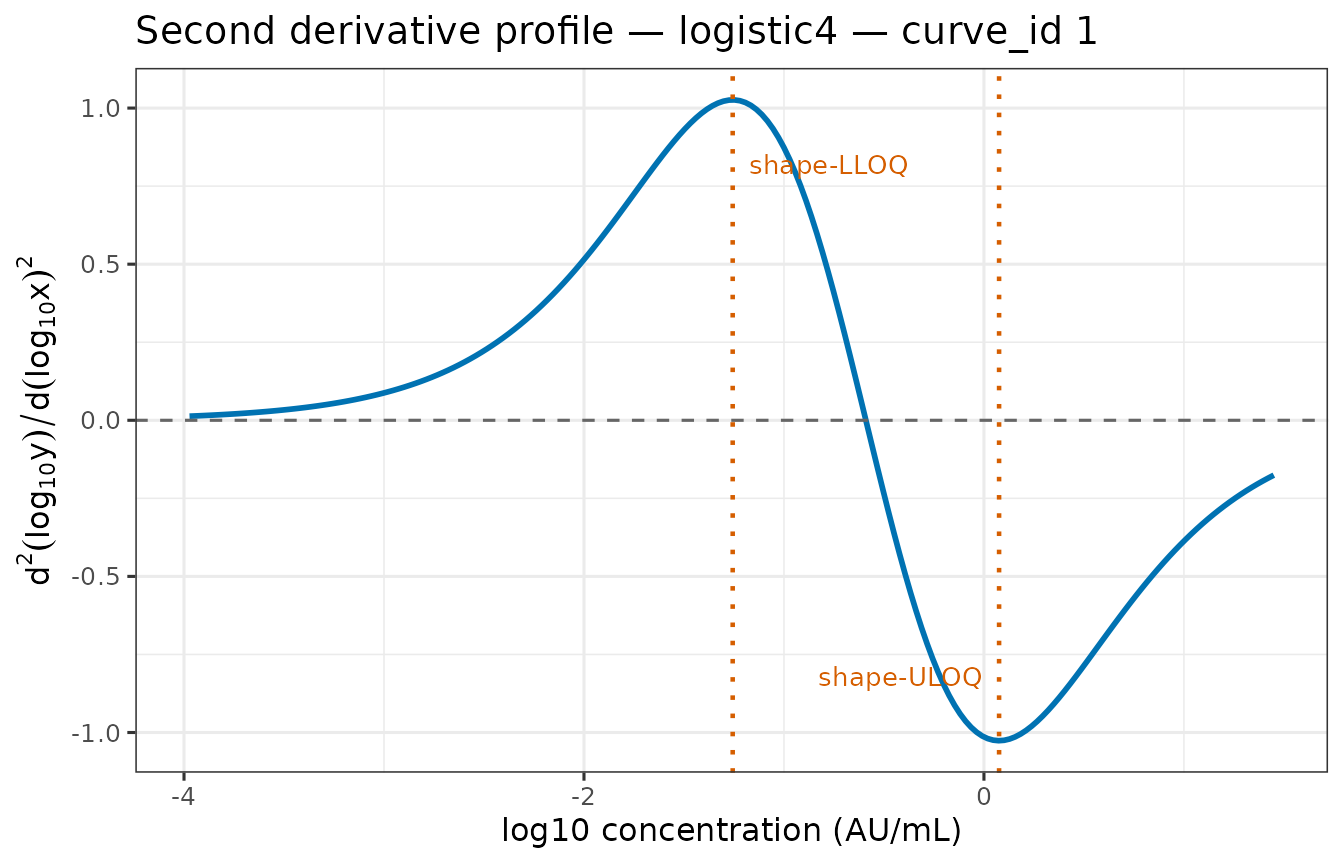
Second derivative profile for the best eligible model (curve_id 1). The peak marks the shape-LLOQ and the valley marks the shape-ULOQ.

Comparing shape-LOQ with pcov-LOQ

shape_vs_pcov <- data.frame(
  Metric          = c("Shape-LLOQ", "Shape-ULOQ", "pcov-LLOQ", "pcov-ULOQ"),
  log10_conc      = c(best_elig$shape_lloq_log10, best_elig$shape_uloq_log10,
                      best_elig$lloq, best_elig$uloq),
  stringsAsFactors = FALSE
)
shape_vs_pcov$conc_AU_mL <- 10^shape_vs_pcov$log10_conc

knitr::kable(shape_vs_pcov, digits = 3,
             caption = paste("Shape-LOQ vs pcov-LOQ for", sel$best_model_name, "(curve_id 1)"))

Shape-LOQ vs pcov-LOQ for logistic4 (curve_id 1)
Metric	log10_conc	conc_AU_mL
Shape-LLOQ	-1.256	0.055
Shape-ULOQ	0.076	1.190
pcov-LLOQ	-1.443	0.036
pcov-ULOQ	0.322	2.098

The shape-LOQ is purely geometric (depends only on curve shape), while the pcov-LOQ incorporates measurement uncertainty. The shape-LOQ typically provides a tighter range.

CI-based detection limits: LOD, MDC, and RDL

The $detection_limits element of each calibration_result contains three families of metrics computed from parameter confidence intervals:

LODs (Limits of Detection): the upper 97.5% CI of a (lower LOD) and the lower 2.5% CI of d (upper LOD), mapped to both the response and concentration scales.
MDC (Minimum Detectable Concentration): the LOD response values inverted through the point-estimate curve.
RDL (Reliable Detection Limits): LOD response values inverted through CI-modified curves (conservative = compressed d; liberal = expanded d).

dl <- cr1$detection_limits

if (!is.null(dl)) {
  dl_summary <- data.frame(
    Metric     = c("Lower LOD", "Upper LOD",
                   "MDC (lower)", "MDC (upper)",
                   "RDL (lower, conservative)", "RDL (upper, liberal)"),
    Response   = c(dl$lods$lower_lod_response,
                   dl$lods$upper_lod_response,
                   NA, NA, NA, NA),
    log10_conc = c(dl$lods$lower_lod_log10_conc,
                   dl$lods$upper_lod_log10_conc,
                   dl$mdc_rdl$mdc_lower_log10,
                   dl$mdc_rdl$mdc_upper_log10,
                   dl$mdc_rdl$rdl_lower_log10,
                   dl$mdc_rdl$rdl_upper_log10),
    conc_AU_mL = c(dl$lods$lower_lod_conc,
                   dl$lods$upper_lod_conc,
                   dl$mdc_rdl$mdc_lower_conc,
                   dl$mdc_rdl$mdc_upper_conc,
                   dl$mdc_rdl$rdl_lower_conc,
                   dl$mdc_rdl$rdl_upper_conc),
    stringsAsFactors = FALSE
  )

  knitr::kable(dl_summary, digits = 4,
               caption = paste("Detection limits for", dl$model_name,
                               "(curve_id 1, alpha =", dl$alpha, ")"))
}

Detection limits for logistic4 (curve_id 1, alpha = 0.05 )
Metric	Response	log10_conc	conc_AU_mL
Lower LOD	1.9045	-1.6864	0.0206
Upper LOD	4.2989	1.4084	25.6093
MDC (lower)	NA	-1.6864	0.0206
MDC (upper)	NA	1.4084	25.6093
RDL (lower, conservative)	NA	-1.6757	0.0211
RDL (upper, liberal)	NA	1.0580	11.4301

All QC limits on one plot

g  <- as.data.frame(cr1$grid)
dl <- cr1$detection_limits

p <- ggplot(g, aes(x = x_fit, y = predicted_response)) +
  geom_line(colour = "#0072B2", linewidth = 1.2)

# pcov-LOQ shaded region
if (is.finite(elig_best$lloq) && is.finite(elig_best$uloq)) {
  p <- p + annotate("rect",
                     xmin = elig_best$lloq, xmax = elig_best$uloq,
                     ymin = -Inf, ymax = Inf,
                     fill = "#009E73", alpha = 0.08) +
    geom_vline(xintercept = c(elig_best$lloq, elig_best$uloq),
               linetype = "dotted", colour = "#009E73", linewidth = 0.7)
}

# Shape-LOQ
if (is.finite(best_elig$shape_lloq_log10))
  p <- p + geom_vline(xintercept = best_elig$shape_lloq_log10,
                       linetype = "dashed", colour = "#D55E00", linewidth = 0.7)
if (is.finite(best_elig$shape_uloq_log10))
  p <- p + geom_vline(xintercept = best_elig$shape_uloq_log10,
                       linetype = "dashed", colour = "#D55E00", linewidth = 0.7)

# LOD horizontal lines
if (!is.null(dl) && is.finite(dl$lods$lower_lod_response))
  p <- p + geom_hline(yintercept = dl$lods$lower_lod_response,
                       colour = "darkorange", linewidth = 0.6)
if (!is.null(dl) && is.finite(dl$lods$upper_lod_response))
  p <- p + geom_hline(yintercept = dl$lods$upper_lod_response,
                       colour = "darkorange", linewidth = 0.6)

# MDC points
if (!is.null(dl) && is.finite(dl$mdc_rdl$mdc_lower_log10))
  p <- p + annotate("point",
                     x = dl$mdc_rdl$mdc_lower_log10,
                     y = dl$lods$lower_lod_response,
                     shape = 17, colour = "darkorange", size = 3)
if (!is.null(dl) && is.finite(dl$mdc_rdl$mdc_upper_log10))
  p <- p + annotate("point",
                     x = dl$mdc_rdl$mdc_upper_log10,
                     y = dl$lods$upper_lod_response,
                     shape = 17, colour = "darkorange", size = 3)

p + labs(x = "log10 concentration (AU/mL)",
         y = "log10(MFI)",
         title = paste("QC metrics overlay —", sel$best_model_name, "— curve_id 1")) +
  theme_bw(base_size = 12)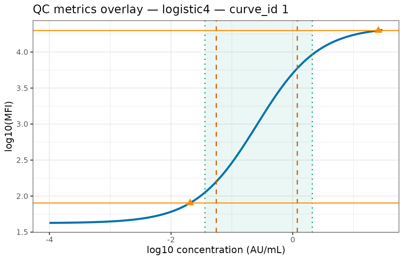

Calibration curve (curve_id 1) with all quantification and detection limits overlaid.

Legend: Green shading = pcov quantifiable range (LLOQ to ULOQ). Orange dashed = shape-LOQ (curvature-based). Orange horizontal lines = LOD response thresholds. Orange triangles = MDC (concentration at LOD response).

Sample back-calculation and final concentrations

How back-calculation works

For each test sample, predict_samples_freq() applies the analytical inverse of the best-fit model to the observed response:

Log-transform the raw response: y_fit = log10(max(mfi, 1e-6)).
Invert the forward model via the closed-form inverse (e.g. for 4PL: $x = c + b \log \frac{y - a}{d - y}$ ) to obtain predicted_concentration on the log10 scale.
Propagate uncertainty via the delta method: $\text{Var}(x) = \nabla_\theta x^\top \Sigma \nabla_\theta x + \left(\frac{\partial x}{\partial y}\right)^2 \sigma_y^2$ , yielding se_concentration and pcov.
Recover pre-dilution concentration: final_concentration = 10^x * dilution.

All analytical inverse and gradient functions reside in curveRcore (inverses.R, gradients.R) and are selected via curveRcore::make_inv_and_grad_fixed(), which returns a list of three closures (inv, grad, grad_y) built once per model and reused across all samples.

Extracting sample predictions

collect_samples() concatenates sample prediction frames across all curves:

all_samples_pred <- collect_samples(mp)
head(all_samples_pred[, c(
  "curve_id", "sampleid", "mfi",
  "predicted_concentration", "final_concentration",
  "se_concentration", "pcov", "pcov_pass"
)])
#>   curve_id sampleid     mfi predicted_concentration final_concentration
#> 1        1     a001 18323.4                1.133390         27190.70184
#> 2        1     a002 19414.7                1.310105         40844.64561
#> 3        1     a003 20098.5                1.453272         56793.90770
#> 4        1     a004 19556.0                1.337046         43458.65254
#> 5        1     a005 20177.5                1.472263         59332.60615
#> 6        1     a006    70.1               -1.817592            30.43951
#>   se_concentration      pcov pcov_pass
#> 1        0.3075734  70.82139      TRUE
#> 2        0.4268163  98.27808      TRUE
#> 3        0.5613527 129.25624      TRUE
#> 4        0.4491785 103.42716      TRUE
#> 5        0.5823824 134.09850      TRUE
#> 6        0.2095433  48.24912      TRUE

Output columns added by `predict_samples_freq()`

Column	Description
`raw_assay_response`	Original response value (e.g. MFI) before any transform.
`observed_response_fit`	Response on the fitting scale (`log10(mfi)` when `is_log_response = TRUE`).
`predicted_log10_concentration`	Back-calculated concentration on the log10 scale.
`predicted_concentration`	Same as `predicted_log10_concentration` when `is_log_independent = TRUE`.
`final_concentration`	Pre-dilution concentration: `10^predicted_concentration × dilution`.
`se_concentration`	Delta-method SE of `predicted_concentration`.
`pcov`	%CV of back-calculated concentration.
`pcov_rmse`	Relative RMSE; for samples equals `pcov` (bias undefined without known truth).
`pcov_pass`	`TRUE` when `pcov < cv_x_max` and finite.

Flagging out-of-range samples

n_total       <- nrow(all_samples_pred)
n_pass        <- sum(all_samples_pred$pcov_pass, na.rm = TRUE)
n_out_of_range <- n_total - n_pass

cat(sprintf("Total samples : %d\n", n_total))
#> Total samples : 120
cat(sprintf("pcov_pass = TRUE : %d  (%.1f %%)\n",
            n_pass, 100 * n_pass / n_total))
#> pcov_pass = TRUE : 84  (70.0 %)
cat(sprintf("Out-of-range    : %d  (%.1f %%)\n",
            n_out_of_range, 100 * n_out_of_range / n_total))
#> Out-of-range    : 36  (30.0 %)

# Convert predicted_concentration (log10 scale) back to natural scale
all_samples_pred$conc_AU_mL <- 10^all_samples_pred$predicted_concentration *
                                 all_samples_pred$dilution

ggplot(all_samples_pred,
       aes(x = factor(curve_id), y = log10(conc_AU_mL),
           colour = pcov_pass)) +
  geom_jitter(width = 0.25, size = 1.5, alpha = 0.8) +
  scale_colour_manual(values = c("TRUE" = "#009E73", "FALSE" = "#CC3311"),
                      labels = c("TRUE" = "Within range",
                                 "FALSE" = "Out of range")) +
  labs(x = "curve_id", y = "log10 final concentration (AU/mL)",
       colour = "pcov_pass",
       title = "Back-calculated concentrations — all curves") +
  theme_bw(base_size = 12)
#> Warning: Removed 7 rows containing missing values or values outside the scale range
#> (`geom_point()`).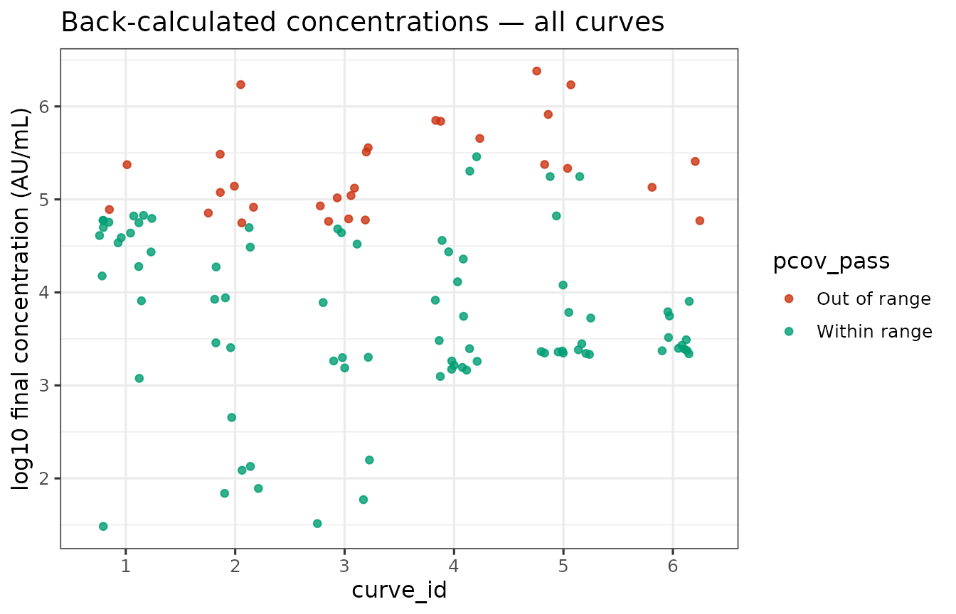

Back-calculated serum concentrations for all samples, coloured by pcov_pass status.

The `calibration_result` object structure

Single-curve object

fit_calibration_freq() returns a calibration_result S3 object (defined in curveRcore). Its components are:

cr1 <- mp$plates[["1"]]
str(cr1, max.level = 1)
#> List of 9
#>  $ meta            :List of 12
#>  $ ensemble        :List of 2
#>  $ selection       :List of 8
#>  $ grid            :'data.frame':    200 obs. of  12 variables:
#>  $ samples         :'data.frame':    20 obs. of  22 variables:
#>  $ diagnostics     : NULL
#>  $ standards       :'data.frame':    10 obs. of  9 variables:
#>  $ blanks          :'data.frame':    4 obs. of  7 variables:
#>  $ detection_limits:List of 5
#>  - attr(*, "class")= chr [1:2] "calibration_result" "list"

Component	Type	Contents
`$meta`	list	Fitting metadata: method, package, version, timestamp, `curve_id`, `response_var`, `is_log_response`, `n_standards`, `n_samples`, `pcov_threshold`.
`$ensemble`	named list	One entry per model name. Each entry contains `model_name`, `converged`, `parameters`, `fit_stats`, `raw_fit`, `grid`, and `eligibility`.
`$selection`	list	`best_model_name`, `criterion`, `fallback`, `fallback_reason`, `assessments`, `eligible_models`, `weights` (AIC table), `aic_best`.
`$grid`	data frame	Precision grid for the best model (pointer to `ensemble[[best]]$grid`).
`$samples`	data frame or NULL	Back-calculated predictions for test samples.
`$standards`	data frame or NULL	Preprocessed standard curve data used to fit this curve, stored for QA and plotting.
`$blanks`	data frame or NULL	Blank measurements for this curve, stored for QA and plotting of the zero-signal reference.

Accessing ensemble entries

# Parameters for the best model
best_nm  <- cr1$selection$best_model_name
cr1$ensemble[[best_nm]]$parameters
#>   term   estimate  std_error
#> 1    a  1.6247987 0.14270068
#> 2    d  4.3501440 0.02615353
#> 3    c -0.5903620 0.06937180
#> 4    b  0.5054454 0.04603846

# Fit statistics
cr1$ensemble[[best_nm]]$fit_stats
#> $n_obs
#> [1] 10
#> 
#> $n_params
#> [1] 4
#> 
#> $df_resid
#> [1] 6
#> 
#> $rss
#> [1] 0.01341037
#> 
#> $aic
#> [1] -27.76435
#> 
#> $bic
#> [1] -26.25142
#> 
#> $log_lik
#> [1] 18.88217

# Raw nlsLM object — all standard S3 methods apply
coef(cr1$ensemble[[best_nm]]$raw_fit)
#>          a          d          c          b 
#>  1.6247987  4.3501440 -0.5903620  0.5054454

Accessing the precision grid for the non-selected model

Since every converged model has a grid, you can inspect precision for the runner-up:

all_models  <- names(cr1$ensemble)
runner_up   <- setdiff(all_models, sel$best_model_name)

if (length(runner_up) > 0 &&
    cr1$ensemble[[runner_up]]$converged) {
  grid_ru <- cr1$ensemble[[runner_up]]$grid
  cat("Runner-up model:", runner_up, "\n")
  cat("Grid rows:", nrow(grid_ru), "\n")
  cat("pcov range: [",
      round(min(grid_ru$pcov, na.rm = TRUE), 1), ",",
      round(max(grid_ru$pcov, na.rm = TRUE), 1), "]\n")
}
#> Runner-up model: gompertz4 
#> Grid rows: 200 
#> pcov range: [ 39.6 , 150 ]

Multi-curve object

fit_calibration_freq_multiplate() wraps results in a calibration_result_multiplate object:

str(mp, max.level = 1)
#> List of 2
#>  $ meta  :List of 8
#>  $ plates:List of 6
#>  - attr(*, "class")= chr [1:2] "calibration_result_multiplate" "list"

Component	Contents
`$meta`	Global metadata: `method`, `package`, `curve_ids`, `n_curves`, `response_var`, timestamp.
`$plates`	Named list of `calibration_result` objects, one per `curve_id`. NULL entries indicate failed curves when `on_error = "warn"`.

Summary extraction helpers

Two helper functions operate on calibration_result_multiplate objects:

# One row per curve: best model, parameters, fit statistics
tbl <- summary_table(mp)
print(tbl[, c("curve_id", "best_model", "converged", "aic", "a", "b", "c", "d")])
#>   curve_id best_model converged         aic           a         b          c
#> 1        1  logistic4      TRUE -27.7643473  1.62479874 0.5054454 -0.5903620
#> 2        2  logistic4      TRUE -19.1687882  1.04897855 0.5884898 -0.7908089
#> 3        3  logistic4      TRUE -24.7379571  1.54079238 0.5074881 -0.6672782
#> 4        4  logistic4      TRUE  -4.1681595 -0.33551913 0.6232312  0.2475139
#> 5        5  gompertz4      TRUE  -0.6238382 -0.06969946 1.4938193  0.1063683
#> 6        6  gompertz4      TRUE  16.9190343  0.44440821 2.0000000  0.1649602
#>          d
#> 1 4.350144
#> 2 4.322849
#> 3 4.358659
#> 4 4.600872
#> 5 4.520710
#> 6 4.378936

# All sample predictions in one data frame
samp_all <- collect_samples(mp)
cat("Total rows:", nrow(samp_all), "\n")
#> Total rows: 120
cat("Columns:", paste(names(samp_all), collapse = ", "), "\n")
#> Columns: curve_id, timeperiod, patientid, well, stype, sampleid, agroup, dilution, pctaggbeads, samplingerrors, mfi, assay_response_variable, assay_independent_variable, raw_assay_response, observed_response_fit, predicted_log10_concentration, predicted_concentration, final_concentration, se_concentration, pcov, pcov_rmse, pcov_pass

Summary

This vignette has walked through the complete curveRfreq workflow:

Ecosystem — curveRfreq is the frequentist fitting engine; it depends on curveRcore for preprocessing, model definitions, inverses, gradients, and the calibration_result class.
Preprocessing — curveRcore::preprocess_standards() transforms concentration and response to the log10 scale and handles blanks and prozone effects before any fitting occurs.
Fitting — fit_calibration_freq_multiplate() splits data by curve_id and fits an ensemble of NLS models per curve.
NLS algorithm — multi-start Levenberg-Marquardt with adaptive bounds; two fallback strategies for low-signal data.
Eligibility gates — four gates (at_bound, vcov_condition, rel_se, dynamic_range) intercept unidentified or boundary-constrained models before AIC ranking.
Audit trail — $selection exposes gate results, the AIC table, fallback status, and the distinction between the AIC winner and the eligibility-gated winner.
Per-model grids — ensemble[[model]]$grid is populated for every converged model and contains the full precision profile (pcov, pcov_rmse, se_concentration).
LLOQ / ULOQ — derived from the precision grid at the pcov_threshold; accessible from ensemble[[model]]$eligibility.
Second derivative and shape-LOQ — d2y_dx2 column on every grid; shape-LLOQ and shape-ULOQ in $eligibility bracket the quasi-linear region of maximum sensitivity.
Detection limits — LODs, MDC, and RDL in $detection_limits, computed from asymptote parameter CIs and the analytical inverse.
Sample back-calculation — analytical inverse + delta-method uncertainty propagation; final_concentration includes the dilution factor; pcov_pass flags whether the sample falls within the quantifiable range.
Object structure — calibration_result is a standard S3 list; summary_table() and collect_samples() extract tidy summaries from multi-curve runs. ```