Model Forms: Mathematics of the Five curveRcore Calibration Models

Forward functions, inverses, derivatives, gradient factory, and prediction grids

---

Introduction

This vignette is a self-contained mathematical reference for the five sigmoidal calibration-curve models implemented in curveRcore. It documents the forward functions, their analytical inverses, first and second derivatives, the gradient-factory used for delta-method error propagation, and the prediction-grid utilities shared by curveRfreq and curveRbayes.

No model fitting is performed here. The audience is a statistician or assay scientist who wants to understand the mathematics before—or independently of—running a full calibration workflow. For a worked end-to-end analysis, see the companion vignette Calibration Curve Workflows.

Notation and conventions

All five models share the following parameter convention, enforced across the entire curveR ecosystem:

Symbol	Role	Constraint
$a$	Lower asymptote (baseline response)	$a < d$
$b$	Scale / slope parameter	$b > 0$
$c$	Inflection-point location on the $x$-axis	real
$d$	Upper asymptote (saturation response)	$d > a$
$g$	Asymmetry parameter (5-parameter models only)	$g > 0$
$x$	Independent variable passed to the model	model-dependent

The independent variable $x$ is scale-agnostic: any monotone transformation (e.g. $x = \log_{10}(\text{concentration})$) is applied upstream in R before the model is called. The models themselves do not perform any transformation internally, except loglogistic4 and loglogistic5, which require $x > 0$ on the raw (un-logged) concentration scale.

---

Forward Model Equations

Four-Parameter Logistic (4PL) — logistic4

$$y = a + \frac{d - a}{1 + \exp\!\left(-\dfrac{x - c}{b}\right)} \tag{4PL}$$

The 4PL is symmetric about its inflection point $(c,\,(a+d)/2)$. It is the workhorse model for log-linear immunoassay standard curves.

# Parameter set used throughout this vignette
p4 <- list(a = 100, b = 0.8, c = 1.5, d = 50000)

x_seq <- seq(-1, 4, length.out = 300)
y_4pl <- logistic4(x_seq, p4$a, p4$b, p4$c, p4$d)

plot(x_seq, y_4pl, type = "l", lwd = 2, col = "#2166AC",
     xlab = expression(log[10](concentration)),
     ylab = "Response (MFI)",
     main = "4PL forward curve")
abline(v = p4$c, h = (p4$a + p4$d) / 2, lty = 2, col = "grey50")
legend("topleft", legend = "logistic4", lwd = 2, col = "#2166AC", bty = "n")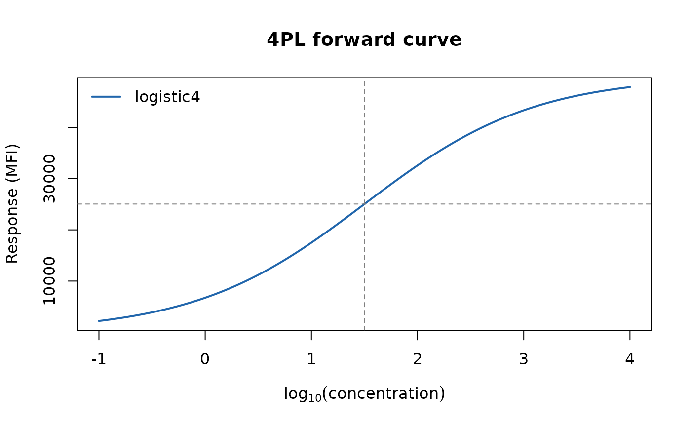

Five-Parameter Logistic (5PL) — logistic5

$$y = a + \frac{d - a}{\left(1 + \exp\!\left(-\dfrac{x - c}{b}\right)\right)^{g}} \tag{5PL}$$

When $g = 1$ this reduces exactly to the 4PL. $g > 1$ compresses the lower shoulder (skews toward the upper asymptote); $0 < g < 1$ compresses the upper shoulder. The inflection point shifts with $g$:

$$x_{\inf} = c + b\ln(g), \qquad y_{\inf} = a + (d-a)\left(\frac{g}{g+1}\right)^{g}$$

p5 <- list(a = 100, b = 0.8, c = 1.5, d = 50000, g = 0.6)

y_5pl <- logistic5(x_seq, p5$a, p5$b, p5$c, p5$d, p5$g)

plot(x_seq, y_4pl, type = "l", lwd = 2, col = "#2166AC", lty = 2,
     xlab = expression(log[10](concentration)),
     ylab = "Response (MFI)",
     main = "4PL vs 5PL (g = 0.6)")
lines(x_seq, y_5pl, lwd = 2, col = "#D6604D")
legend("topleft",
       legend = c("logistic4 (g = 1)", "logistic5 (g = 0.6)"),
       lwd = 2, col = c("#2166AC", "#D6604D"), lty = c(2, 1), bty = "n")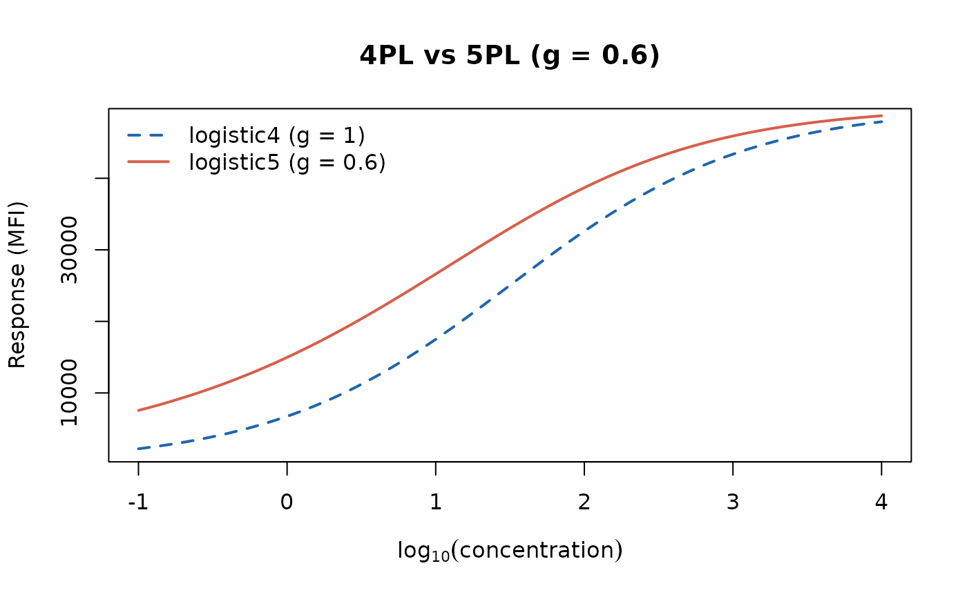

Four-Parameter Log-Logistic — loglogistic4

$$y = a + \frac{d - a}{1 + (c / x)^{b}} \tag{LL4}$$

Here $c > 0$ is the EC50 on the raw concentration scale, and $b$ is the Hill coefficient. This is the classical Hill equation / dose-response parameterisation. Domain restriction: requires $x > 0$. When working on the $\log_{10}$ scale, logistic4 is algebraically equivalent and preferred.

p_ll4 <- list(a = 100, b = 1.8, c = 30, d = 50000)  # c is EC50 in AU/mL
x_conc <- seq(0.01, 500, length.out = 500)

y_ll4 <- loglogistic4(x_conc, p_ll4$a, p_ll4$b, p_ll4$c, p_ll4$d)

plot(log10(x_conc), y_ll4, type = "l", lwd = 2, col = "#4DAC26",
     xlab = expression(log[10](concentration)),
     ylab = "Response (MFI)",
     main = "Log-logistic 4PL — concentration scale")
abline(v = log10(p_ll4$c), lty = 2, col = "grey50")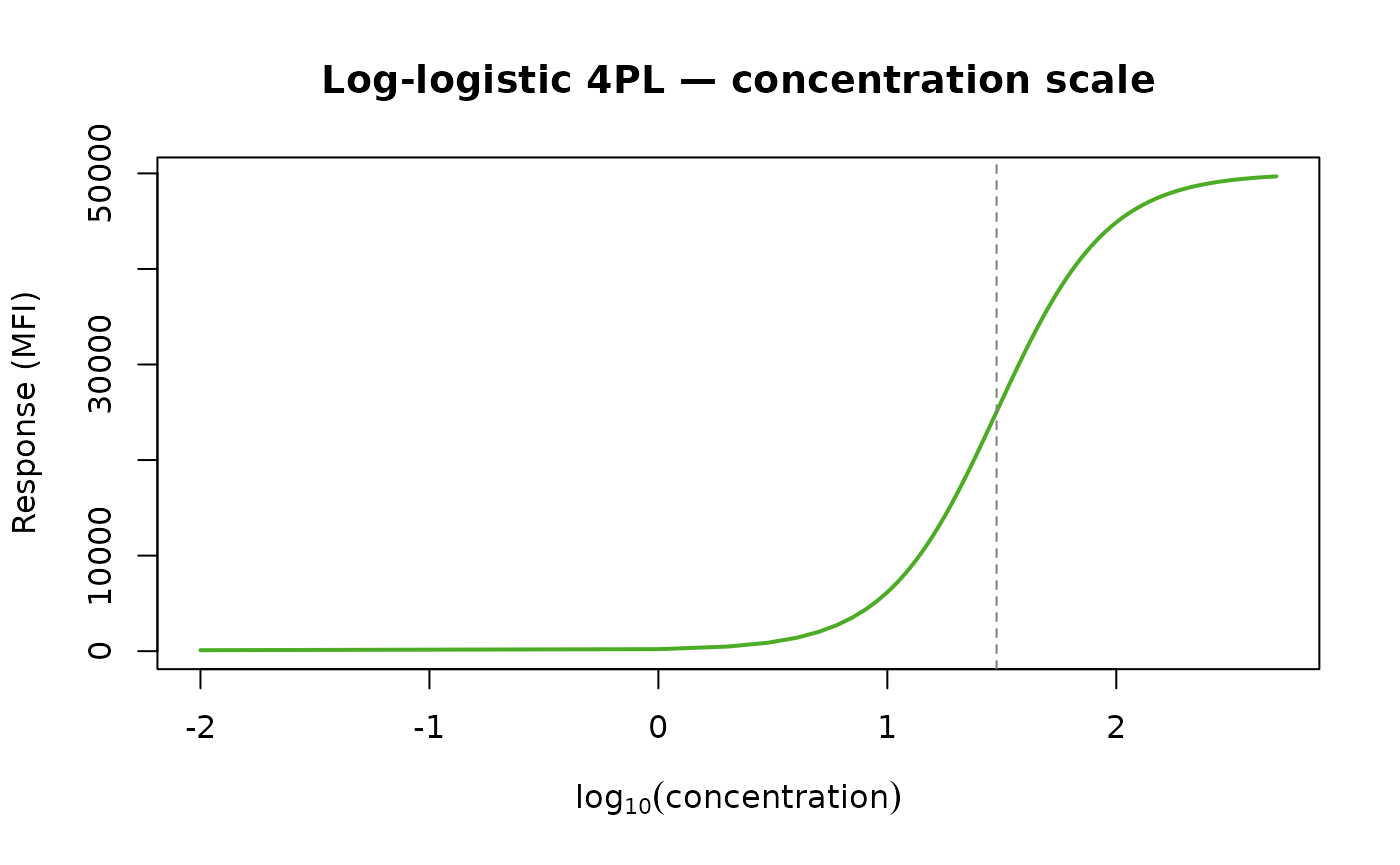

Five-Parameter Generalised Logistic (Richards) — loglogistic5

$$y = a + (d - a)\,\bigl(1 + g\,\exp(-b(x - c))\bigr)^{-1/g} \tag{LL5}$$

This is the Richards / generalised logistic curve (Richards 1959). Despite the name loglogistic5, $x$ here is the log-transformed concentration (i.e. the model operates on the log scale). When $g \to 0$ the formula approaches the Gompertz; when $g = 1$ it matches the 4PL up to a parameter rescaling.

p_ll5 <- list(a = 100, b = 1.2, c = 1.5, d = 50000, g = 0.5)

y_ll5 <- loglogistic5(x_seq, p_ll5$a, p_ll5$b, p_ll5$c, p_ll5$d, p_ll5$g)

plot(x_seq, y_ll5, type = "l", lwd = 2, col = "#762A83",
     xlab = expression(log[10](concentration)),
     ylab = "Response",
     main = "loglogistic5 (Richards / generalised logistic)")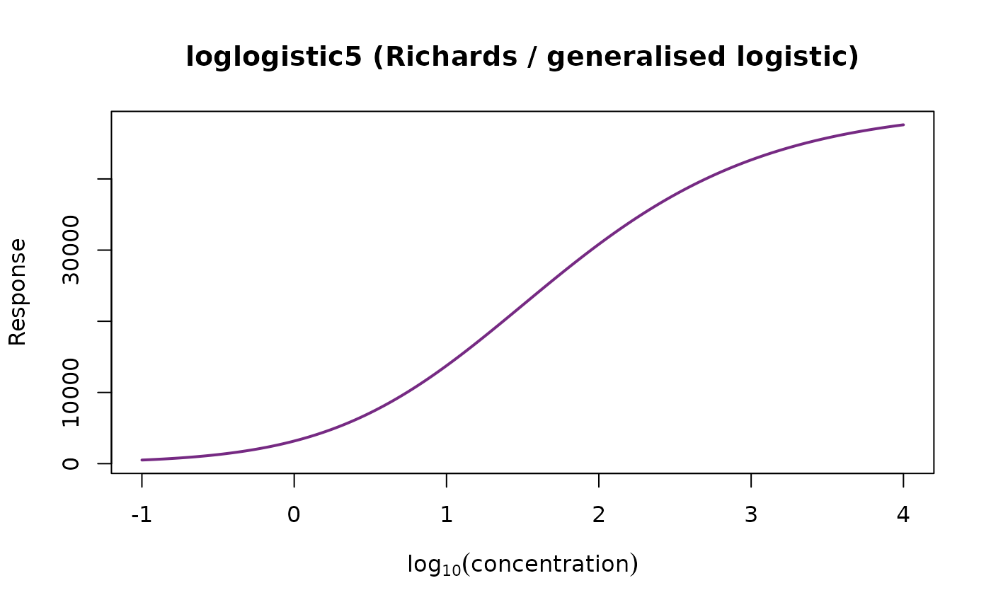

Four-Parameter Gompertz — gompertz4

$$y = a + (d - a)\,\exp\!\bigl(-\exp(-b(x - c))\bigr) \tag{G4}$$

The Gompertz is intrinsically asymmetric: it rises steeply from the lower asymptote and approaches the upper asymptote more gradually (Gompertz 1825). The inflection occurs at $x = c$, where $y_{\inf} = a + (d-a)/e$.

p_g4 <- list(a = 100, b = 1.2, c = 1.5, d = 50000)

y_g4 <- gompertz4(x_seq, p_g4$a, p_g4$b, p_g4$c, p_g4$d)

plot(x_seq, y_4pl,  type = "l", lwd = 2, col = "#2166AC", lty = 2,
     xlab = expression(log[10](concentration)),
     ylab = "Response",
     main = "4PL vs Gompertz — asymmetry comparison")
lines(x_seq, y_g4, lwd = 2, col = "#BF812D")
abline(v = p_g4$c, lty = 3, col = "grey60")
legend("topleft",
       legend = c("logistic4 (symmetric)", "gompertz4 (asymmetric)"),
       lwd = 2, col = c("#2166AC", "#BF812D"), lty = c(2, 1), bty = "n")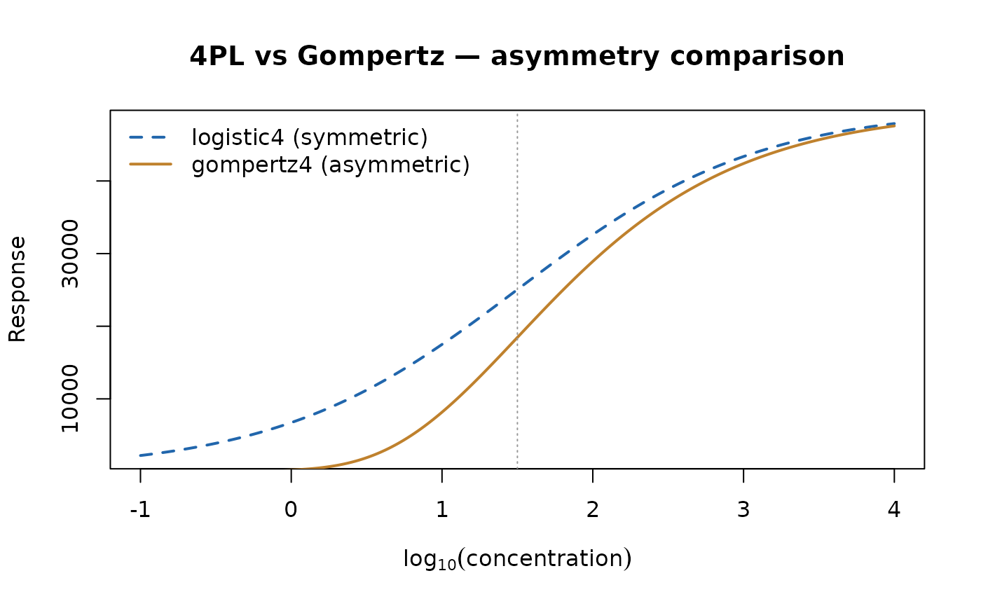

Summary comparison table

Model	Equation kernel	Symmetry	Parameters	x domain
logistic4	$(1 + e^{-(x-c)/b})^{-1}$	Symmetric	$a,b,c,d$	$\mathbb{R}$
logistic5	$(1 + e^{-(x-c)/b})^{-g}$	Asymmetric	$a,b,c,d,g$	$\mathbb{R}$
loglogistic4	$(1 + (c/x)^b)^{-1}$	Symmetric	$a,b,c,d$	$x > 0$
loglogistic5	$(1 + g\,e^{-b(x-c)})^{-1/g}$	Asymmetric	$a,b,c,d,g$	$\mathbb{R}$
gompertz4	$\exp(-e^{-b(x-c)})$	Asymmetric	$a,b,c,d$	$\mathbb{R}$

---

Analytical Inverse Functions

Each model has a closed-form inverse that maps an observed response $y$ back to the concentration scale. Two variants exist for every model:

• inv_<model>(y, a, b, c, d) — $a$ is a free (estimated) parameter.
• inv_<model>_fixed(y, fixed_a, b, c, d) — $a$ is supplied as an external constant (e.g. from a plate blank mean), reducing Monte Carlo uncertainty.

All functions return NA for $y$ values outside the open interval $(a, d)$.

Inverse formulae

4PL inverse

Solving $y = a + (d-a)/(1 + e^{-(x-c)/b})$ for $x$:

$$x = c + b\,\ln\!\frac{y - a}{d - y} \tag{inv-4PL}$$

5PL inverse

$$x = c - b\,\ln\!\left(\left(\frac{d - a}{y - a}\right)^{1/g} - 1\right) \tag{inv-5PL}$$

Log-logistic 4PL inverse

$$x = \frac{c}{\displaystyle\left(\frac{d - y}{y - a}\right)^{1/b}} \tag{inv-LL4}$$

Log-logistic 5PL inverse

$$x = c - \frac{1}{b}\,\ln\!\frac{\left(\dfrac{y-a}{d-a}\right)^{-g} - 1}{g} \tag{inv-LL5}$$

Gompertz inverse

$$x = c - \frac{1}{b}\,\ln\!\left(-\ln\frac{y - a}{d - a}\right) \tag{inv-G4}$$

Worked example: round-trip verification

A useful sanity check is to confirm $x = f^{-1}(f(x))$ to machine precision.

x_true <- 2.0  # log10(100 AU/mL)

# ---- 4PL ----
y_fwd  <- logistic4(x_true, p4$a, p4$b, p4$c, p4$d)
x_back <- inv_logistic4(y_fwd, p4$a, p4$b, p4$c, p4$d)
cat(sprintf("4PL   round-trip error: %.2e\n", abs(x_back - x_true)))
#> 4PL   round-trip error: 0.00e+00

# ---- 5PL ----
y_fwd  <- logistic5(x_true, p5$a, p5$b, p5$c, p5$d, p5$g)
x_back <- inv_logistic5(y_fwd, p5$a, p5$b, p5$c, p5$d, p5$g)
cat(sprintf("5PL   round-trip error: %.2e\n", abs(x_back - x_true)))
#> 5PL   round-trip error: 0.00e+00

# ---- loglogistic4 ----
x_ll4  <- log10(100)  # = 2.0; x_conc must be positive
y_fwd  <- loglogistic4(100, p_ll4$a, p_ll4$b, p_ll4$c, p_ll4$d)
x_back <- inv_loglogistic4(y_fwd, p_ll4$a, p_ll4$b, p_ll4$c, p_ll4$d)
cat(sprintf("LL4   round-trip error: %.2e\n", abs(x_back - 100)))
#> LL4   round-trip error: 1.42e-14

# ---- loglogistic5 ----
y_fwd  <- loglogistic5(x_true, p_ll5$a, p_ll5$b, p_ll5$c, p_ll5$d, p_ll5$g)
x_back <- inv_loglogistic5(y_fwd, p_ll5$a, p_ll5$b, p_ll5$c, p_ll5$d, p_ll5$g)
cat(sprintf("LL5   round-trip error: %.2e\n", abs(x_back - x_true)))
#> LL5   round-trip error: 0.00e+00

# ---- Gompertz ----
y_fwd  <- gompertz4(x_true, p_g4$a, p_g4$b, p_g4$c, p_g4$d)
x_back <- inv_gompertz4(y_fwd, p_g4$a, p_g4$b, p_g4$c, p_g4$d)
cat(sprintf("G4    round-trip error: %.2e\n", abs(x_back - x_true)))
#> G4    round-trip error: 4.44e-16

All errors should be at or below $10^{-12}$, confirming numerical consistency between the forward and inverse functions.

Effect of fixing $a$ on back-calculated concentration

When the lower asymptote $a$ is fixed at a known value (e.g. the mean of blank wells), the resulting inverse uses fewer estimated parameters and yields narrower confidence intervals.

# Suppose we know the blank mean is 95 MFI
a_fixed <- 95
y_test  <- 10000  # an observed sample MFI

x_free  <- inv_logistic4(y_test, p4$a, p4$b, p4$c, p4$d)
x_fixed <- inv_logistic4_fixed(y_test, a_fixed, p4$b, p4$c, p4$d)

cat(sprintf("Back-calculated x (a free):  %.4f\n", x_free))
#> Back-calculated x (a free):  0.3829
cat(sprintf("Back-calculated x (a fixed): %.4f\n", x_fixed))
#> Back-calculated x (a fixed): 0.3833

---

Derivatives

First derivatives (dy/dx)

All first derivatives are positive when $b > 0$ and $a < d$, confirming strict monotonicity.

4PL — dydx_logistic4

Let $u = \exp(-(x-c)/b)$. Then:

$$\frac{dy}{dx} = \frac{(d-a)\,u}{b\,(1+u)^2} \tag{D1-4PL}$$

The maximum slope occurs at $x = c$ (the inflection point), where $u = 1$:

$$\left.\frac{dy}{dx}\right|_{x=c} = \frac{d - a}{4b} \tag{D1-4PL-inf}$$

5PL — dydx_logistic5

$$\frac{dy}{dx} = \frac{g\,(d-a)\,u}{b\,(1+u)^{g+1}} \tag{D1-5PL}$$

The 5PL inflection is at $x_{\inf} = c + b\ln g$, so the maximum slope is:

$$\left.\frac{dy}{dx}\right|_{x=x_{\inf}} = \frac{(d-a)\,g^{g/(g+1) - 1/g}}{b\,(1 + g^{-1})^{g+1}}$$

Log-logistic 4PL — dydx_loglogistic4

Let $r = (c/x)^b$. Then:

$$\frac{dy}{dx} = \frac{b\,(d-a)\,r}{x\,(1+r)^2} \tag{D1-LL4}$$

The inflection on the raw scale is at $x = c$, where $r = 1$:

$$\left.\frac{dy}{dx}\right|_{x=c} = \frac{d-a}{4c}$$

Log-logistic 5PL — dydx_loglogistic5

Let $u = 1 + g\,e^{-b(x-c)}$. Then:

$$\frac{dy}{dx} = b\,(d-a)\,e^{-b(x-c)}\,u^{-1/g - 1} \tag{D1-LL5}$$

Gompertz — dydx_gompertz4

Let $v = \exp(-b(x-c))$. Then:

$$\frac{dy}{dx} = b\,(d-a)\,v\,\exp(-v) \tag{D1-G4}$$

The Gompertz inflection is at $x = c$ ($v = 1$):

$$\left.\frac{dy}{dx}\right|_{x=c} = \frac{b\,(d-a)}{e}$$

Second derivatives (d²y/dx²)

Second derivatives locate the inflection points and characterise the curvature of each shoulder. Analytical forms exist for the 4PL and Gompertz; numerical central-difference approximations are used for the three remaining models.

4PL (analytical) — d2x_logistic4

$$\frac{d^2y}{dx^2} = -\frac{(d-a)\,u\,(1-u)}{b^2\,(1+u)^3} \tag{D2-4PL}$$

At $x = c$ ($u = 1$) the second derivative is zero, confirming the inflection.

Gompertz (analytical) — d2x_gompertz4

$$\frac{d^2y}{dx^2} = b^2\,(d-a)\,v\,(v-1)\,\exp(-v) \tag{D2-G4}$$

At $x = c$ ($v = 1$): $d^2y/dx^2 = 0$. Consistent with $x = c$ being the Gompertz inflection point.

5PL, LL4, LL5 (numerical) — d2x_logistic5, d2x_loglogistic4, d2x_loglogistic5

For models where closed-form second derivatives are algebraically unwieldy, a symmetric central-difference scheme is used with step size $h = 10^{-5}$:

$$\frac{d^2y}{dx^2}\bigg|_x \approx \frac{f(x+h) - 2f(x) + f(x-h)}{h^2}$$

This yields $O(h^2)$ accuracy; for typical parameter magnitudes the approximation error is below $10^{-7}$.

Worked example: slope at an arbitrary point and at the inflection

x_eval <- 2.0  # evaluate at log10(100) AU/mL

# ---- 4PL first derivative ----
slope_4pl <- dydx_logistic4(x_eval, p4$a, p4$b, p4$c, p4$d)
slope_inf  <- (p4$d - p4$a) / (4 * p4$b)   # analytical inflection slope
cat(sprintf("4PL  dy/dx at x=2.0  : %.2f MFI / log10-unit\n", slope_4pl))
#> 4PL  dy/dx at x=2.0  : 14164.85 MFI / log10-unit
cat(sprintf("4PL  dy/dx at x=c=%.1f: %.2f (formula: (d-a)/(4b))\n",
            p4$c, slope_inf))
#> 4PL  dy/dx at x=c=1.5: 15593.75 (formula: (d-a)/(4b))

# ---- Gompertz first derivative at inflection ----
slope_g4     <- dydx_gompertz4(p_g4$c, p_g4$a, p_g4$b, p_g4$c, p_g4$d)
slope_g4_inf <- p_g4$b * (p_g4$d - p_g4$a) / exp(1)
cat(sprintf("\nGompertz dy/dx at inflection (x=c): %.2f\n", slope_g4))
#> 
#> Gompertz dy/dx at inflection (x=c): 22028.62
cat(sprintf("Gompertz formula b*(d-a)/e        : %.2f\n", slope_g4_inf))
#> Gompertz formula b*(d-a)/e        : 22028.62

# ---- Visualise slope profile across the curve ----
slopes_4pl  <- dydx_logistic4(x_seq, p4$a, p4$b, p4$c, p4$d)
slopes_g4   <- dydx_gompertz4(x_seq, p_g4$a, p_g4$b, p_g4$c, p_g4$d)

par(mfrow = c(1, 2), mar = c(4, 4, 3, 1))

plot(x_seq, slopes_4pl, type = "l", lwd = 2, col = "#2166AC",
     xlab = expression(x == log[10](conc)),
     ylab = "dy/dx  (MFI / log10-unit)",
     main = "4PL slope profile")
abline(v = p4$c, lty = 2, col = "grey50")

plot(x_seq, slopes_g4, type = "l", lwd = 2, col = "#BF812D",
     xlab = expression(x == log[10](conc)),
     ylab = "dy/dx  (MFI / log10-unit)",
     main = "Gompertz slope profile")
abline(v = p_g4$c, lty = 2, col = "grey50")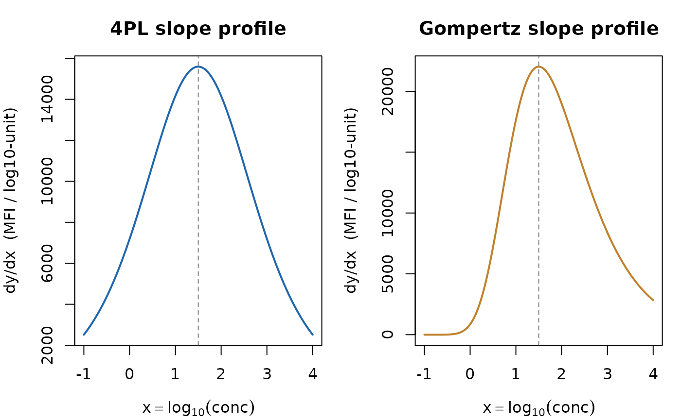

par(mfrow = c(1, 1))

# Confirm d²y/dx² = 0 at the 4PL inflection
d2_at_inf <- d2x_logistic4(p4$c, p4$a, p4$b, p4$c, p4$d)
cat(sprintf("4PL d²y/dx² at inflection: %.2e  (expect 0)\n", d2_at_inf))
#> 4PL d²y/dx² at inflection: -0.00e+00  (expect 0)

# Numerical second derivative for the 5PL
d2_5pl_at_c <- d2x_logistic5(p5$c, p5$a, p5$b, p5$c, p5$d, p5$g)
cat(sprintf("5PL d²y/dx² at x=c      : %.4f\n", d2_5pl_at_c))
#> 5PL d²y/dx² at x=c      : -3086.3885
# Note: the 5PL inflection is at x = c + b*log(g), not at x = c
x_inf_5pl <- p5$c + p5$b * log(p5$g)
d2_5pl_at_xinf <- d2x_logistic5(x_inf_5pl, p5$a, p5$b, p5$c, p5$d, p5$g)
cat(sprintf("5PL d²y/dx² at x_inf=%.3f: %.2e  (expect ~0)\n",
            x_inf_5pl, d2_5pl_at_xinf))
#> 5PL d²y/dx² at x_inf=1.091: 3.64e-02  (expect ~0)

---

Gradient Factory: make_inv_and_grad_fixed

Purpose

Delta-method confidence intervals for back-calculated concentrations require three quantities for each observed response $y$:

1. $\hat{x} = f^{-1}(y;\,\hat\theta)$ — the point estimate.
2. $\nabla_\theta\, x = \partial x/\partial \theta$ — sensitivity of $x$ to each model parameter.
3. $\partial x/\partial y$ — sensitivity of $x$ to measurement error in $y$.

The uncertainty in $\hat{x}$ is then:

$$\operatorname{Var}(\hat{x}) \approx \bigl(\nabla_\theta\, x\bigr)^\top \,\mathbf{V}_{\hat\theta}\, \bigl(\nabla_\theta\, x\bigr) \;+\; \left(\frac{\partial x}{\partial y}\right)^2\!\sigma_y^2 \tag{DeltaVar}$$

where $\mathbf{V}_{\hat\theta} = \operatorname{Cov}(\hat\theta)$ is the parameter covariance matrix and $\sigma_y^2$ is the assay noise variance at $y$.

API

fns <- make_inv_and_grad_fixed(model, fixed_a = NULL)

Arguments

• model — character string, one of "logistic4", "logistic5", "loglogistic4", "loglogistic5", "gompertz4".
• fixed_a — numeric scalar or NULL. If non-NULL, $a$ is treated as a known constant and excluded from $\nabla_\theta\, x$, typically reducing the number of free parameters from 4 (or 5) to 3 (or 4).

Return value

A list of three closures, each with signature function(y, p) where p is the named vector returned by coef(fit):

Closure	Returns
$inv(y, p)	Scalar $\hat x$
$grad(y, p)	Named numeric vector $\nabla_\theta\, x$
$grad_y(y, p)	Scalar $\partial x/\partial y$

Analytical gradient formulae

4PL

Using $x = c + b\ln\!\left(\frac{y-a}{d-y}\right)$:

$$\frac{\partial x}{\partial a} = \frac{-b}{y-a}, \quad \frac{\partial x}{\partial b} = \ln\frac{y-a}{d-y}, \quad \frac{\partial x}{\partial c} = 1, \quad \frac{\partial x}{\partial d} = \frac{-b}{d-y}$$

$$\frac{\partial x}{\partial y} = \frac{b\,(d-a)}{(y-a)(d-y)}$$

5PL

Let $T = (d-a)/(y-a)$, $T_g = T^{1/g}$, $W = T_g - 1$:

$$\frac{\partial x}{\partial a} = \frac{b\,T_g}{g\,W\,(y-a)}, \quad \frac{\partial x}{\partial b} = -\ln W, \quad \frac{\partial x}{\partial c} = 1, \quad \frac{\partial x}{\partial d} = \frac{-b\,T_g}{g\,W\,(d-a)}$$

$$\frac{\partial x}{\partial g} = \frac{b\,T_g\,\ln T}{g^2\,W}, \quad \frac{\partial x}{\partial y} = \frac{-b\,T_g}{g\,W\,(y-a)}$$

Log-logistic 4PL

Let $Q = (d-y)/(y-a)$, $p = 1/b$, $x = c/Q^p$:

$$\frac{\partial x}{\partial a} = \frac{-c p\,(d-y)\,Q^{-p-1}}{(y-a)^2}, \quad \frac{\partial x}{\partial b} = \frac{x\,\ln Q}{b^2}, \quad \frac{\partial x}{\partial c} = Q^{-p}, \quad \frac{\partial x}{\partial d} = c p\,Q^{-p-1}/(y-a)$$

$$\frac{\partial x}{\partial y} = \frac{c p\,(d-a)\,Q^{-p-1}}{(y-a)^2}$$

Gompertz

Let $R = (y-a)/(d-a)$, $L = -\ln R > 0$:

$$\frac{\partial x}{\partial a} = \frac{1}{b\,L\,(y-a)}, \quad \frac{\partial x}{\partial b} = \frac{\ln L}{b^2}, \quad \frac{\partial x}{\partial c} = 1, \quad \frac{\partial x}{\partial d} = \frac{-1}{b\,L\,(d-a)}$$

$$\frac{\partial x}{\partial y} = \frac{1}{b\,L\,(y-a)}$$

Log-logistic 5PL

Let $\rho = (y-a)/(d-a)$, $\rho_g = \rho^{-g}$, $V = \rho_g - 1$:

$$\frac{\partial x}{\partial a} = \frac{\rho^{-g-1}}{b\,g\,V\,(d-a)}, \quad \frac{\partial x}{\partial b} = \frac{\ln V - \ln g}{b^2}, \quad \frac{\partial x}{\partial c} = 1$$

$$\frac{\partial x}{\partial d} = \frac{\rho^{-g-1}(y-a)}{b\,g\,V\,(d-a)^2}, \quad \frac{\partial x}{\partial g} = \frac{1 - \ln(g V)}{b\,g^2}$$

$$\frac{\partial x}{\partial y} = \frac{\rho^{-g-1}}{b\,g\,V\,(d-a)}$$

Worked example: gradient factory in action

# Simulate a coefficient vector as would come from coef(fit)
p_hat <- c(a = 100, b = 0.8, c = 1.5, d = 50000)

# Build the closure set for 4PL with a estimated freely
fns_free <- make_inv_and_grad_fixed("logistic4", fixed_a = NULL)

y_obs <- 15000  # observed MFI

x_hat  <- fns_free$inv(y_obs, p_hat)
g_hat  <- fns_free$grad(y_obs, p_hat)
gy_hat <- fns_free$grad_y(y_obs, p_hat)

cat(sprintf("Back-calculated log10(conc): %.4f\n", x_hat))
#> Back-calculated log10(conc): 0.8168
cat("Gradient w.r.t. theta:\n")
#> Gradient w.r.t. theta:
print(round(g_hat, 5))
#>        a        b        c        d 
#> -0.00005 -0.85399  1.00000 -0.00002
cat(sprintf("Gradient w.r.t. y: %.6f\n", gy_hat))
#> Gradient w.r.t. y: 0.000077

# ---- Verify against finite differences ----
eps <- 1e-6
fd_grad <- sapply(names(p_hat), function(nm) {
  p_up       <- p_hat
  p_up[[nm]] <- p_hat[[nm]] + eps
  (fns_free$inv(y_obs, p_up) - x_hat) / eps
})
cat("\nFinite-difference check (should match grad above):\n")
#> 
#> Finite-difference check (should match grad above):
print(round(fd_grad, 5))
#>        a        b        c        d 
#> -0.00005 -0.85399  1.00000 -0.00002

# ---- With fixed_a ----
fns_fixed <- make_inv_and_grad_fixed("logistic4", fixed_a = 95)
g_fixed   <- fns_fixed$grad(y_obs, p_hat[c("b", "c", "d")])
cat("\nGradient with fixed a=95 (b, c, d only):\n")
#> 
#> Gradient with fixed a=95 (b, c, d only):
print(round(g_fixed, 5))
#>        b        c        d 
#> -0.85365  1.00000 -0.00002

Applying the delta-method variance formula

# A toy parameter covariance matrix (realistic order-of-magnitude)
V_theta <- diag(c(a = 4, b = 0.002, c = 0.01, d = 250000))
rownames(V_theta) <- colnames(V_theta) <- names(p_hat)

sigma_y <- 200   # assay CV ≈ 1.3% at MFI=15000

var_x_param <- as.numeric(t(g_hat) %*% V_theta %*% g_hat)
var_x_meas  <- gy_hat^2 * sigma_y^2
var_x_total <- var_x_param + var_x_meas

cat(sprintf("Variance from parameter uncertainty: %.5f (log10 units^2)\n",
            var_x_param))
#> Variance from parameter uncertainty: 0.01159 (log10 units^2)
cat(sprintf("Variance from measurement noise    : %.5f\n", var_x_meas))
#> Variance from measurement noise    : 0.00023
cat(sprintf("Total variance in back-calculated x: %.5f\n", var_x_total))
#> Total variance in back-calculated x: 0.01182
cat(sprintf("95%% CI half-width: ± %.4f log10 units\n",
            qnorm(0.975) * sqrt(var_x_total)))
#> 95% CI half-width: ± 0.2131 log10 units

---

Prediction Grid Utilities

generate_prediction_grid

The prediction grid is a data frame of concentration values at which the fitted curve and its confidence band are evaluated for plotting and interpolation. Both curveRfreq and curveRbayes use the same grid structure, ensuring visual consistency.

generate_prediction_grid(
  std_curve_conc,
  n_grid             = 200L,
  grid_min_conc      = 1e-4,
  grid_max_conc      = NULL,
  is_log_independent = TRUE
)

Key arguments

• std_curve_conc — the maximum standard concentration (AU/mL). When grid_max_conc = NULL, this value is used as the upper boundary.
• n_grid — number of evenly-spaced grid points. Default 200 gives smooth curves without excessive computation.
• grid_min_conc — lower boundary of the grid on the raw scale. Must be $> 0$.
• is_log_independent — if TRUE (default), grid points are evenly spaced on the $\log_{10}$ scale, matching the fitting scale for log-transformed models; if FALSE, points are evenly spaced on the linear concentration scale.

Return value

A data frame with three columns:

Column	Description
log10_concentration	$\log_{10}$ of concentration
concentration	Concentration on the raw (AU/mL) scale
x_fit	The value actually passed to the model ($= \log_{10}c$ when is_log_independent = TRUE)

predict_grid_response

Evaluates the forward model at every grid point:

predict_grid_response(grid, model_name, params)

Returns a numeric vector of $\hat y$ values of length n_grid.

Worked example: building and plotting a prediction grid

# Generate a 300-point log-scale grid from 0.0001 to 30 AU/mL
grid <- generate_prediction_grid(
  std_curve_conc = 30,
  n_grid         = 300,
  grid_min_conc  = 1e-4,
  is_log_independent = TRUE
)

cat("Grid dimensions:", nrow(grid), "×", ncol(grid), "\n")
#> Grid dimensions: 300 × 3
cat("x_fit range    :", round(range(grid$x_fit), 3), "\n")
#> x_fit range    : -4 1.477
cat("conc range     :", signif(range(grid$concentration), 3), "AU/mL\n")
#> conc range     : 1e-04 30 AU/mL

# Evaluate all five models on the grid
params_4pl  <- c(a = 100, b = 0.8, c = 1.5, d = 50000)
params_5pl  <- c(a = 100, b = 0.8, c = 1.5, d = 50000, g = 0.6)
params_ll4  <- c(a = 100, b = 1.8, c = 30,  d = 50000)
params_ll5  <- c(a = 100, b = 1.2, c = 1.5, d = 50000, g = 0.5)
params_g4   <- c(a = 100, b = 1.2, c = 1.5, d = 50000)

yhat_4pl  <- predict_grid_response(grid, "logistic4",    params_4pl)
yhat_5pl  <- predict_grid_response(grid, "logistic5",    params_5pl)
yhat_ll5  <- predict_grid_response(grid, "loglogistic5", params_ll5)
yhat_g4   <- predict_grid_response(grid, "gompertz4",    params_g4)

# For loglogistic4 the grid x_fit must be on the raw (positive) scale
grid_lin <- generate_prediction_grid(
  std_curve_conc = 500, n_grid = 300,
  grid_min_conc = 0.01, is_log_independent = FALSE
)
yhat_ll4 <- predict_grid_response(grid_lin, "loglogistic4", params_ll4)

cols <- c("4PL"  = "#2166AC", "5PL"  = "#D6604D",
          "LL5"  = "#762A83", "G4"   = "#BF812D")

plot(grid$x_fit, yhat_4pl, type = "l", lwd = 2, col = cols["4PL"],
     xlab = expression(log[10](concentration~~"(AU/mL)")),
     ylab = "Response (MFI)",
     main = "Prediction grids — all five models",
     ylim = c(0, 55000))
lines(grid$x_fit, yhat_5pl,  lwd = 2, col = cols["5PL"])
lines(grid$x_fit, yhat_ll5,  lwd = 2, col = cols["LL5"])
lines(grid$x_fit, yhat_g4,   lwd = 2, col = cols["G4"])
lines(log10(grid_lin$concentration), yhat_ll4,
      lwd = 2, col = "#4DAC26", lty = 2)

legend("topleft", bty = "n", lwd = 2,
       legend = c("logistic4", "logistic5 (g=0.6)", "loglogistic5 (g=0.5)",
                  "gompertz4", "loglogistic4"),
       col    = c(cols, "#4DAC26"),
       lty    = c(1, 1, 1, 1, 2))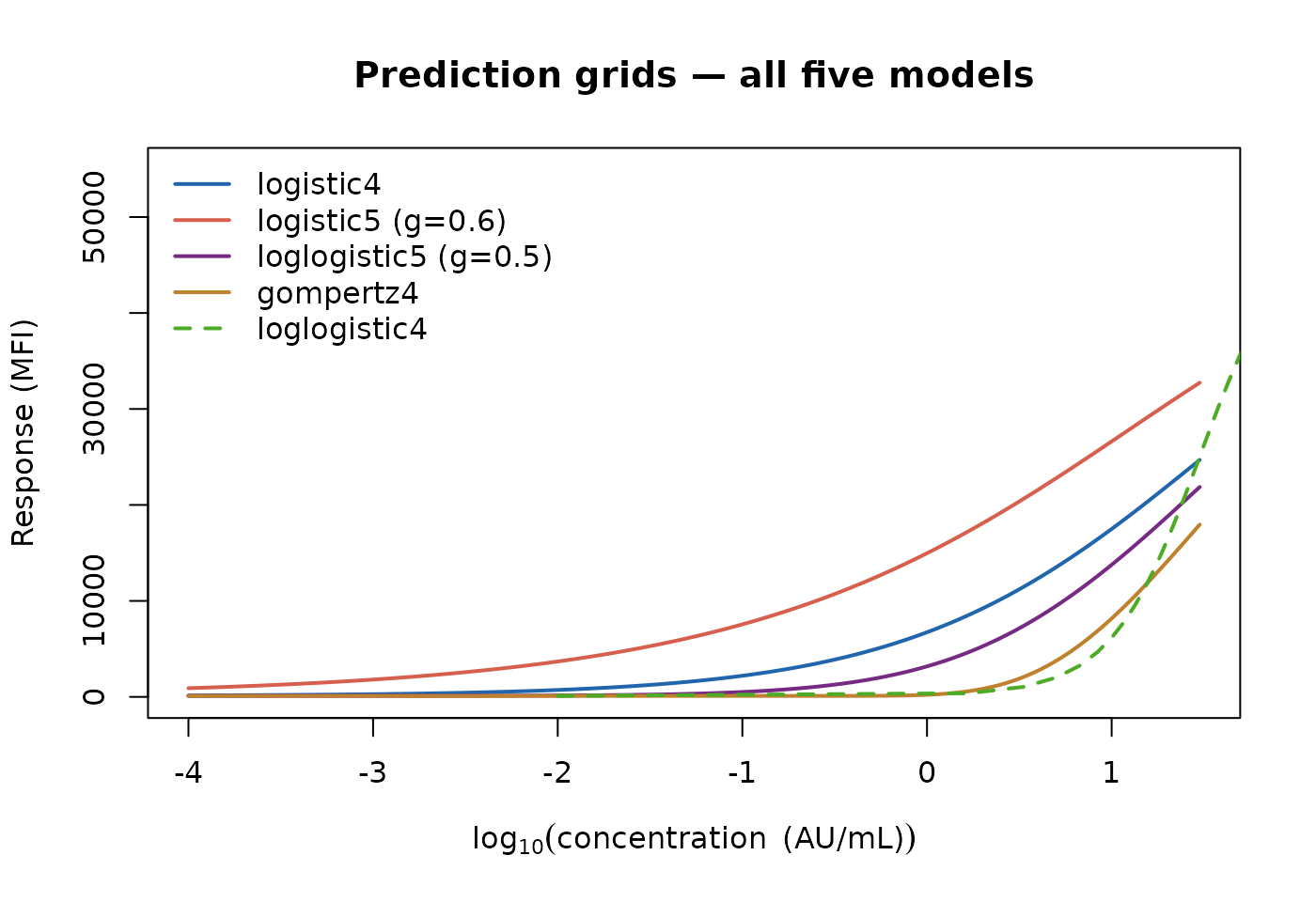

Using the grid for back-calculation across a response range

# Demonstrate back-calculation at a sequence of response values
y_targets <- seq(500, 45000, by = 2000)

x_back <- inv_logistic4(y_targets, params_4pl["a"], params_4pl["b"],
                        params_4pl["c"], params_4pl["d"])

result <- data.frame(
  MFI            = y_targets,
  log10_conc     = round(x_back, 4),
  conc_AU_mL     = round(10^x_back, 3)
)
print(result)
#>      MFI log10_conc conc_AU_mL
#> 1    500    -2.3546      0.004
#> 2   2500    -0.8882      0.129
#> 3   4500    -0.3689      0.428
#> 4   6500    -0.0332      0.926
#> 5   8500     0.2220      1.667
#> 6  10500     0.4324      2.706
#> 7  12500     0.6147      4.118
#> 8  14500     0.7782      6.000
#> 9  16500     0.9286      8.484
#> 10 18500     1.0699     11.746
#> 11 20500     1.2049     16.029
#> 12 22500     1.3359     21.672
#> 13 24500     1.4647     29.156
#> 14 26500     1.5931     39.182
#> 15 28500     1.7227     52.804
#> 16 30500     1.8552     71.651
#> 17 32500     1.9928     98.348
#> 18 34500     2.1378    137.332
#> 19 36500     2.2935    196.564
#> 20 38500     2.4646    291.453
#> 21 40500     2.6580    455.020
#> 22 42500     2.8858    768.770
#> 23 44500     3.1708   1481.812

---

Model Selection Considerations

The table below summarises the key mathematical properties that should guide model choice for a given assay.

Property	4PL	5PL	LL4	LL5	Gompertz
Inflection symmetry	Symmetric	Asymmetric	Symmetric	Asymmetric	Asymmetric (fixed)
Inflection at $x = c$?	Yes	Only if $g=1$	Yes	No	Yes
Extra shape parameter	No	Yes ($g$)	No	Yes ($g$)	No
Closed-form $d^2y/dx^2$	Yes	No	No	No	Yes
Raw-scale $x$ required	No	No	Yes	No	No
Typical application	Log-linear ELISA	Asymmetric ELISA	Hill-equation dose–response	Flexible dose–response	Left-skewed saturation

Practical guidance:

• Start with logistic4. It has the fewest parameters and closed-form derivatives.
• If the residuals show systematic skew in one shoulder, add the asymmetry parameter ($g$) via logistic5.
• Use loglogistic4 / loglogistic5 when you prefer to work on the raw concentration scale (e.g. for pharmacological IC50 reporting).
• gompertz4 is a natural choice for bead-based multiplex assays where the response rises steeply from a low baseline and saturates slowly.

---

Numerical Precision Notes

1. Step size for numerical second derivatives. The default $h = 10^{-5}$ gives $O(h^2) \approx 10^{-10}$ truncation error for parameters of order unity. Reduce $h$ if parameter magnitudes exceed $10^4$.

2. Asymptote guard in inverse functions. inv_logistic4 and inv_logistic5 apply a tolerance buffer of $10^{-6}$ and return NA for responses within that distance of either asymptote, where the logit transformation diverges.

3. Overflow protection in Gompertz. The data-generation helper in bead_assay_example.R caps the exponent $u = b(\ln x - \ln c)$ at 30 to prevent exp(exp(u)) overflow for extreme concentrations; the core gompertz4 function does not apply this cap.

4. Machine precision of round-trips. As demonstrated in Section @ref(sec-inverses), forward–inverse round-trips return errors at the level of $\sim 10^{-13}$, consistent with IEEE 754 double-precision arithmetic.

---

References

Gompertz, B. 1825. “On the Nature of the Function Expressive of the Law of Human Mortality, and on a New Mode of Determining the Value of Life Contingencies.” Philosophical Transactions of the Royal Society of London 115: 513–83. https://doi.org/10.1098/rstl.1825.0026.

Richards, F. J. 1959. “A Flexible Growth Function for Empirical Use.” Journal of Experimental Botany 10 (2): 290–301. https://doi.org/10.1093/jxb/10.2.290.

---

Session Information

sessionInfo()
#> R version 4.6.0 (2026-04-24)
#> Platform: x86_64-pc-linux-gnu
#> Running under: Ubuntu 24.04.4 LTS
#> 
#> Matrix products: default
#> BLAS:   /usr/lib/x86_64-linux-gnu/openblas-pthread/libblas.so.3 
#> LAPACK: /usr/lib/x86_64-linux-gnu/openblas-pthread/libopenblasp-r0.3.26.so;  LAPACK version 3.12.0
#> 
#> locale:
#>  [1] LC_CTYPE=C.UTF-8       LC_NUMERIC=C           LC_TIME=C.UTF-8       
#>  [4] LC_COLLATE=C.UTF-8     LC_MONETARY=C.UTF-8    LC_MESSAGES=C.UTF-8   
#>  [7] LC_PAPER=C.UTF-8       LC_NAME=C              LC_ADDRESS=C          
#> [10] LC_TELEPHONE=C         LC_MEASUREMENT=C.UTF-8 LC_IDENTIFICATION=C   
#> 
#> time zone: UTC
#> tzcode source: system (glibc)
#> 
#> attached base packages:
#> [1] stats     graphics  grDevices utils     datasets  methods   base     
#> 
#> other attached packages:
#> [1] curveRcore_0.2.0
#> 
#> loaded via a namespace (and not attached):
#>  [1] digest_0.6.39     desc_1.4.3        R6_2.6.1          fastmap_1.2.0    
#>  [5] xfun_0.58         cachem_1.1.0      knitr_1.51        htmltools_0.5.9  
#>  [9] rmarkdown_2.31    lifecycle_1.0.5   cli_3.6.6         sass_0.4.10      
#> [13] pkgdown_2.2.0     textshaping_1.0.5 jquerylib_0.1.4   systemfonts_1.3.2
#> [17] compiler_4.6.0    tools_4.6.0       ragg_1.5.2        bslib_0.11.0     
#> [21] evaluate_1.0.5    yaml_2.3.12       otel_0.2.0        jsonlite_2.0.0   
#> [25] rlang_1.2.0       fs_2.1.0

---